How do you find cost and revenue functions?
All businesses produce some kind of product. That product may be something that you can hold in your hand like an MP3 player or it may be a service like cleaning an office. The outputs from the business take the form of goods and services. To produce these outputs, the business requires inputs such as workers, machines and supplies. A business takes the inputs and converts them to outputs.
The process of converting inputs to outputs requires technology. This is more than our everyday meaning where we think of technology as a cool new product or technique. In economics, technology is any process a business uses to convert inputs into outputs. It depends on many factors. For instance, in a dairy the factors might include the capacity of the milking machinery, the skill of the laborers who operate the machinery and the quality of the feed the cows are fed.
Technological change may occur if the businesses inputs and outputs change. This can occur in two basic ways. First, there may be a change in the outputs for the same number of inputs. If greater output occurs for the same level of inputs, positive technological change has occurred. If lower output occurs for the same level of input, negative technological change has taken place. For instance, if a dairy produces more milk with the same number of cows, positive technological change has taken place.
Technological change can also take place if the outputs are held constant and the inputs change. Positive technological change occurs if the same output occurs, but from a lower level of inputs. On the other hand, negative technological change occurs if the same outputs occur for an increased level of inputs. If a dairy produces the same amount of milk from fewer cows, positive change has taken place. If it takes more cows to produce the same level of milk, negative change has taken case.
Businesses are interested in knowing the relationship between the inputs and outputs with respect to the costs they incur to produce the outputs. Since there can be many different inputs that affect their costs, at least one of the businesses input are held constant. This period of time is called the short run. The period of time for which any of the businesses inputs can vary or it can change its technology or capacity is called the long run.
Let’s consider several inputs for a dairy that could lead to the output of milk. A dairy could change the number of cows producing milk, the number of breeding cows, the number of laborers, the capacity of the milking machines, the type of feed or the number of acres used to graze the cows on. The long run is the period of time over which the dairy can vary all of these inputs. The short run is the period of time over which at least one of the inputs is fixed. If the number of cows producing milk is varied over a year, but all other inputs are fixed, the short run is a year. Depending on what is fixed and what is left to vary influences the short run.
To examine the total cost of producing outputs, it is often easiest to look at the short run and to fix as many of the inputs as possible. If only one variable changes, the total cost function will contain only one variable. A total cost function with two variables means that two inputs are varied and so on.
Costs typically fall into two categories, variable costs and fixed costs. To determine which category a cost falls, we need to examine how the cost changes as the outputs change. If a cost varies as the output changes, the cost is a variable cost. A cost that does not change as the output changes is a fixed cost. For a dairy, the labor costs, veterinary costs, feed costs, and utility costs change as the output level of milk changes. To produce more milk, more people need to feed and milk the cows. More milk also means that it will cost more to maintain the health of the herd as well as to operate the milking machines. Costs like real estate taxes, interest on short term loans, and depreciation on equipment are fixed as milk production changes and would be considered fixed costs. All costs are either variable or fixed.
The total cost of operating the business is the sum of the variable costs and the fixed costs,
Total Cost = Fixed Cost + Variable Cost
For a cost function in which all inputs are fixed except one, a single variable is used and the cost function is called C(Q) or Cost(Q). The variable Q is the input that is varied and needs to be defined so that the function makes sense.
Example 4 Dairy Costs
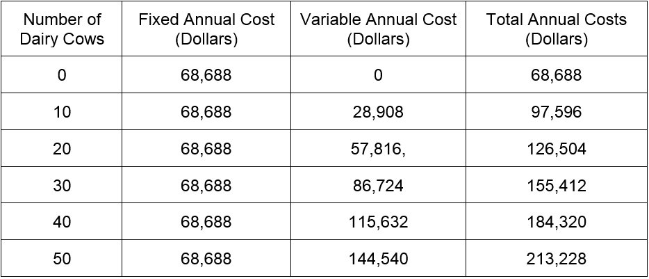
Use Table 2 to find a function that describes the total annual costs C(Q) of running a dairy as a function of the number of cows Q producing milk. By saying “annual”, we are assuming that the short run is a period of one year. Since the function C(Q) has only one input Q, all others are being held constant in the short run.
The table below describes the fixed, variable and total costs as the number of dairy cows is increased.
Table 2
Solution Notice that in each row of Table 2, the total cost is the sum fixed cost and the variable cost.
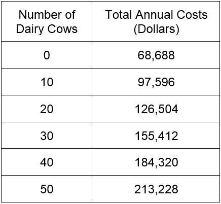
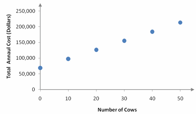
Let’s get a feel for C(Q) by graphing the pertinent columns of this table in a scatter plot. The variable Q represents the number of dairy cows so this will be the input or independent variable on the scatter plot. The dependent variable represents the total cost. This means that we’ll graph the first and fourth columns of the table as ordered pairs,
The scatter plot of the ordered pairs is shown below.
Figure 7 – Scatter plot of data in Table 2
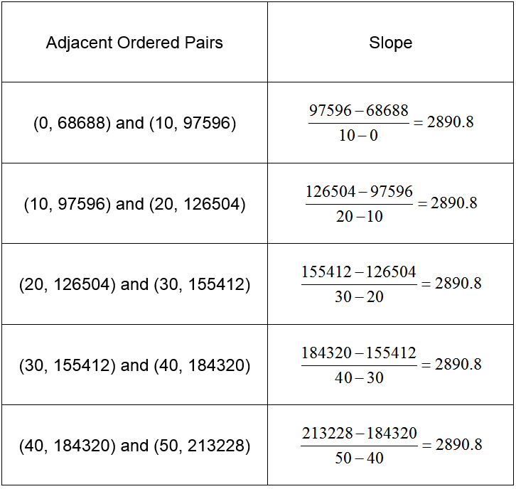
The ordered pairs appear to follow a straight line. To check, let’s calculate the slope between adjacent points on the graph.
Adjacent sets of points have the same slope, 2890.8, so all points lie along a line.
The slope of the line is 2890.8 and the vertical intercept is 68688. Since the graph corresponds to a linear function, we can write the total cost function as
C(Q) = 2890.8Q + 68688
where Q is the number of dairy cows. The term 68688 is fixed as Q changes and corresponds to the fixed costs.
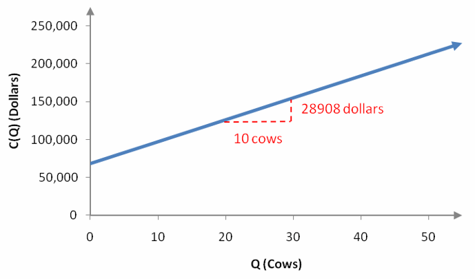
Figure 8 – The linear function corresponding to the data in Figure 7.
The slope indicates the rate at which costs are changing. In this case, we can think of the slope as
This tells us that increasing the number of cows by one increases the total cost by 2890.8 dollars. Thus the variable term 2890.8Q corresponds to the variable cost since the term changes as Q changes.
The slope is also called the marginal cost since it describes how the costs change when the input changes by 1 unit. In general, the term marginal describes how one quantity changes when the input changes by 1 unit.
As discussed before, businesses convert inputs to outputs. This process costs businesses money which is described by the total cost function C(Q). To compensate for these costs, businesses receive money for selling goods or services. The amount received depends on the inputs to the businesses and is called revenue. The revenue function is denoted by the name R or the name Revenue and is a function of the company’s inputs. Typically revenue is described in the short term where at least one of the inputs is fixed. If all but one of the inputs are fixed, the revenue can be denoted by a function of one variable R(Q) or Revenue(Q).
Example 5 Dairy Revenue
A dairy can increase its milk production and thus its revenue in several ways. By changing the feed or administering certain hormones, the amount of milk produced can be increased and lead to higher total revenue. Revenue can also be changed by increasing or decreasing the number of dairy cows. More cows can produce more milk thus leading to higher revenue. We are interested in varying the number of cows Q and seeing how the total annual revenue R(Q) changes. All other inputs to the business will be held constant in the short run.
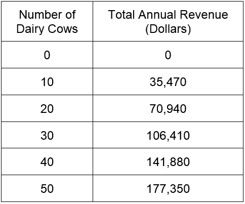
The table below describes the level of total annual revenue for various numbers of dairy cows.
Table 4
Find the revenue function R(Q).
Solution This is a function of the number of dairy cows. On a graph, we know that the number of dairy cows will be graphed horizontally and the total annual cost will be graphed vertically.
Figure 9 – Scatter plot of data in Table 4.
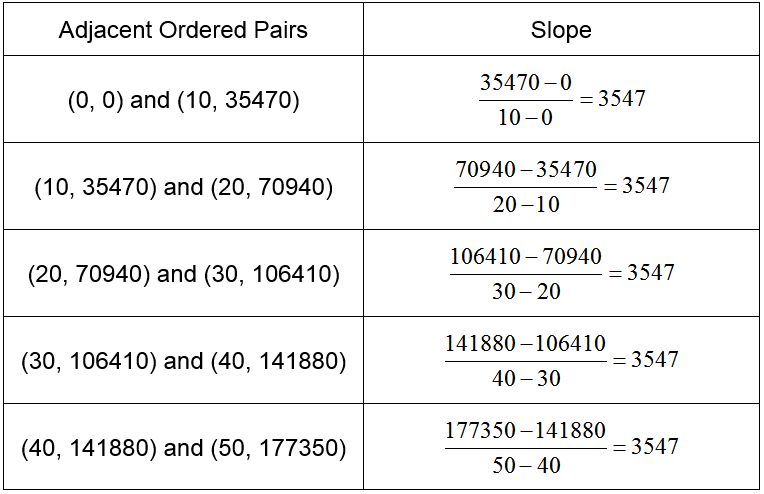
Like the total annual cost, the total annual revenue appears to follow a straight line. Let’s calculate the slope between adjacent points.
Table 5
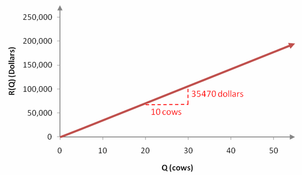
The slope between any pair of points on the line is 3547. This indicates that the ordered pairs all lie along a line that has a slope of 3547. Since the vertical intercept of this line is the point (0,0), we can use the slope-intercept form of a line to write
R(Q) = 3547Q
The graph of this function mirrors the trend of the data in the scatter plot above.
Figure 10 – The linear function corresponding to the data in Figure 9.
We can think of the slope of the revenue function as a ratio,
An increase in the number of dairy cows by 10 leads to an increase in revenue of $35,470. This means that each additional dairy cow adds $3547 to the revenue. The amount of revenue added when the input increases by one unit is called the marginal revenue.
