Section 2.4 Question 3

How do you use row operations to determine the reduced row echelon form of a matrix?

To solve a system of linear equations using matrices, we must convert the augmented matrix to another matrix that is in reduced row echelon form.

 

Each of the augmented matrices below is in reduced row echelon form:

When an augmented matrix is in reduced row echelon form, it is easy to find the solution to the system of linear equations.

 

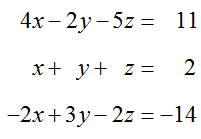
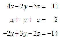
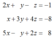
For instance, suppose we have the system of linear equations

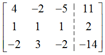
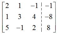
This system yields the augmented matrix

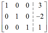
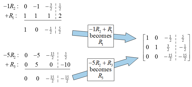
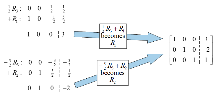
Later in this section we see how to get the reduced row echelon form for this matrix,

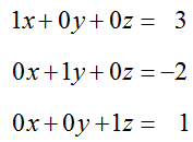
If we rewrite this matrix as a system of linear equations, we get

Dropping all of the terms with a 0 coefficient leads to the solution, x = 3, y = -2, and z = 1.

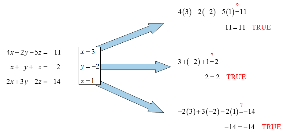
We can check to see that these values satisfy the original system to insure it is equivalent to the system of equations corresponding to the reduced row echelon form:

To solve a system of m linear equations in n variables, we will follow a simple strategy.

 

An augmented matrix is transformed to its reduced row echelon form by using three different operations on the rows. These row operations change the entries in the rows without changing the solutions to the corresponding system of linear equations. If these operations seem familiar, it is no mistake. Each operation corresponds to an equation transformation discussed in Section 2.2.

 

Our goal is to use these row operations to transform the original augmented matrix to its reduced row echelon form.

It is helpful to symbolize the row operations to help identify what is being done. If we want to interchange two rows like the first and second, we will write

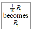
To symbolize that a row is being multiplied by a constant and replacing another row we use a similar notation. For instance, if we want to indicate that row 1 is being replaced by ¹/₁₀ of row 1 we would write

If we need to indicate that multiples of rows are being added and replacing another row, we would write something like

This particular notation indicates that you are multiplying row 2 by -2 and adding it to row 3. The sum is placed in the third row. Notes like these help us to document our row operations. You are encouraged to adopt the same notes so that you can follow your own work easily.

Example 4    Solve a System of Linear Equations Using Matrices

Solve the system of equations

by transforming its augmented matrix to reduced row echelon form.

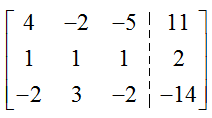
Solution The augmented matrix for this system is

The strategy for finding its reduced row echelon form is similar to the strategy for the Elimination Method.

To put this matrix into reduced row echelon form, we’ll work with each column, one at a time. Instead of using equation transformations to change the leading coefficient to a 1, we’ll use row operations to create a 1 in the entry in the first row and first column of the matrix. After placing the 1, we’ll use row operations to put zeros in the rest of the column. This step corresponds to eliminating the first variable in all of the equations except the first equation. We’ll continue through the rest of the columns of the matrix placing ones and zeros in a manner similar to the Elimination Method.

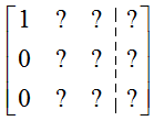
First we’ll use row operations to transform the original augmented matrix to

In each column we’ll use row operations to put the 1 in the column and then continue to use row operations so that the zeros appear below the 1. The 1 is called the pivot in the column.

For this augmented matrix, we could multiply the first row by ¹/₄ or interchange the first and second rows. If we multiply the first row by ¹/₄ and replace the first row with the result we get

The symbols on the left indicate that each entry in the first row is multiplied by ¹/₄.

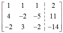
If we interchange the first and second rows we get

Either row operation puts a 1 at the top of the first column. However, interchanging the rows does not introduce any fractions into the problem, so that is the best row operation to use.

Now that the pivot has been established, we’ll use it to put zeros everywhere else in the column. To put a 0 below the one, multiply the first row by -4 and add the result to the second row. Place the sum in the second row:

The symbols on the left show -4 times the first row of the matrix and the second row below it.  Adding the columns vertically gives the sum that is placed underneath the horizontal bar. The blue arrow indicates where that sum is placed in the matrix.

To put a 0 in the bottom of the first column, multiply the first row in this new matrix by 2 and add it to the third row. Place the sum in the third row:

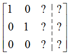
The first column is in the proper format so now we continue onto the second column. We need to use more row operations to change this new matrix into

Start by putting a 1 in the middle of the second column. This can be done in many ways, but we multiply the second row by –¹/₆ to place the pivot. This gives us

With the pivot in place, we now put zeros in the rest of the second column:

Next we place the pivot in the third column. To put a 1 in the bottom of the third column, multiply the third row by –²/₁₅  and place the result in the third column:

Now that the pivot has been established in the third column, we can place zeros in the rest of the column.

This matrix is in reduced row echelon form and indicates that the solution is x = 3, y = -2, and z = 1.

---

 

Example 5    Solve a System of Linear Equations Using Matrices

Solve the system of equations

by transforming its augmented matrix to reduced row echelon form.

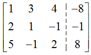
Solution The augmented matrix for this system is

To place a 1 at the top of the first column, interchange the first and second rows. This transforms the original augmented matrix to

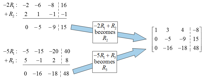
A zero is created below the pivot by multiplying the first row by -2, adding this to the second row, and placing the result in the second row. A zero is also created at the bottom of the first column by multiplying the first row by -5, adding this to the third row, and placing the result in the third row. These two row operations yield

In the second column, we need to place a pivot (a 1) in the second row. Multiply the second row by –¹/₅ and place the result in the second row:

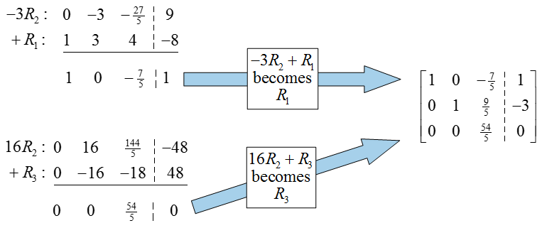
Once the pivot is established, we can use it to put zeros in the rest of the column:

With these two row operations, the second column is in the proper format for reduced row echelon form. In the third column, we need to place a pivot in the third row. To do this, multiply the third row by ⁵/₅₄ :

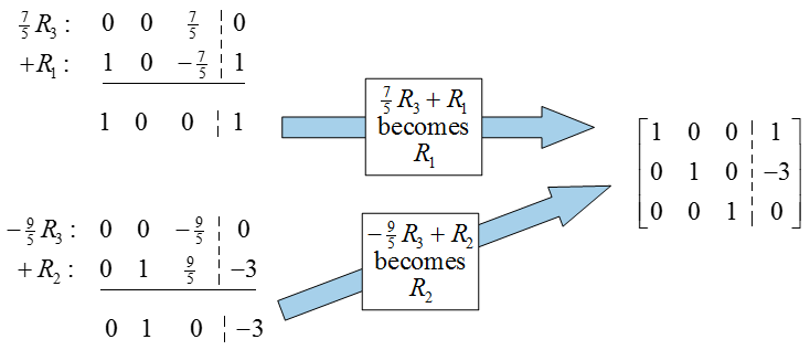
Create zeros above the pivot to put the matrix in reduced row echelon form:

Since the first column corresponds to x, the second column to y and the third column to z, the solution to the original system is x = 1, y = -3, and z = 0.

---

 

In each of the last two examples, the same strategy is used to find the reduced row echelon form. Starting with the first column, we place the pivot in the proper position by interchanging rows or multiplying a row by a constant. Once the pivot is in place, we can multiply the pivot row by a constant and add it to the other rows to put zeros in the rest of the column. By doing this in each column, we can efficiently get the reduced row echelon form and the solution to the system of linear equations.