
How will changes in a constraint’s constant change the optimal solution?
To help us answer this question, let’s develop a new application. Unlike earlier applications of the Simplex Method, this application will be an oversimplified example to make the sensitivity analysis easier to understand. Once we have developed and solved this application, we’ll examine how the optimal solution changes when we change the constants on the right hand side of the constraints.
Example 1 Solve the Standard Maximization Problem
A custom manufacturer of bicycle accessories produces two types of bags which can be mounted on a bicycle. Frame bags are mounted in the interior frame of a bicycle, and panniers are mounted on a rack over the rear wheel of a bicycle. Each of these products is built to the measurements of the customer’s bicycle and involves a large outlay of employee labor.
The manufacturer has enough materials on hand to produce a total of 35 frame bags and panniers each week. Several employees produce these products. Two employees are able to dedicate 75 hours each week to cut the fabric for these products, and two other employees are able to dedicate 60 hours each week to assembling and packing the products.
Each frame bag takes employees one hour to cut the fabric and two hours to assemble and package. Each pannier takes employees three hours to cut the fabric and one hour to assemble and package. If the profit from each frame bag is $70 and the profit from each pannier is $120, how many units of each product should the manufacturer accept to insure that profit is maximized?
Solution Assume this manufacturer can pick and choose which orders to accept so that it is able to maximize profit by allocating its resources most efficiently. The basic question we must answer is how many frame bags and how many panniers will be produced so that the profit is as large as possible? This indicates the variables should be defined as
x: the number of frame bags produced each week
y: the number of panniers produced each week
Each frame bag generates $70 of profit, and each pannier generates $120 of profit. We can use this information to write the total profit P as
P = 70x + 120y
If the amount of materials and labor is unlimited, the manufacturer can produce an unlimited number of frame bags and panniers for an unlimited amount of profit.
However, this manufacturer has a limited amount of materials and labor available. The total number of frame bags and panniers that can be produced in a week is 35. Since the variables describe the individual numbers of each product, we know that
x + y ≤ 35
The total number of labor hours available for cutting fabric is 75 hours. This total relates to the individual amounts of time required to cut frame bags (1 hour per frame bag) and panniers (3 hours per pannier). By multiplying the amounts per product by the variables, we get the amount of cutting time for x frame bags, 1x, and the amount of cutting time for y panniers, 3y. The constraint
x + 3y ≤ 75
indicates that the total amount time required to cut the material must be less than or equal to 75 hours.
The same type of reasoning for assembly and packaging yields the constraint
2x + y ≤ 60
Putting the constraints and objective function together with non-negativity constraints yields the standard maximization problem,
The initial simplex tableau for this linear programming problem is
The pivot for this matrix is the 3 in the second row and second column. To change this entry to a 1, multiply the second row by 1/3:
To complete the first iteration of the Simplex Method, we need to use row operations to fill the rest of the second column with zeros.
Since the indicator row contains a negative entry in the first column, we need to choose a new pivot.
The first column is the pivot column. Let’s examine the quotients to determine the pivot row:
The lowest quotient, 15, is formed from the last column and the pivot column occurs in the first row so we’ll pick the pivot to be the 2/3 . Multiply the pivot row by 3/2 to create a 1 in the first row, first column:
Next, use row operations to create zeros below the pivot.
Since the indicator row contains no negative numbers, we can use this tableau to read the optimal solution.
If we cover the nonbasic variables,
we see that the optimal solution is x = 15, y = 20. This means the largest profit, $3450, occurs when 15 frame bags and 20 panniers are produced each week.
Since this problem contains two decision variables x and y, we can also solve this problem graphically.
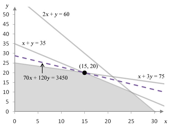
Figure 1 – The feasible region for Example 1.
Figure 1 shows the feasible region corresponding to the constraints for the linear programming problem. The dashed line corresponds to the isoprofit at P = 3450. Any profit higher than $3450 pushes the isoprofit outside of the feasible region, and any lower pushes it inside the feasible region. The solution pictured here, (15, 20), is the greatest profit in the feasible region.
In Example 1, the Simplex Method and the graphical method for solving the linear programming problem both indicate that 15 frame bags and 20 panniers should be produced to achieve a maximum profit of $3450. The question we want to examine now is what would happen if the linear programming problem were changed slightly. For instance, what would happen if the constants in any of the constraints were to change?
Questions such as this one often arise in business applications since the values in the linear programming problem are estimates. Estimates are subject to error or changing values if operating conditions change for the business. An example would be if another person was utilized to help produce frame bags and panniers. This would clearly impact the number of hours that would be available for cutting, assembly and packaging. Will this change the optimal solution? Will it increase or decrease the profit?
To answer these questions, let’s change the constant in the second constraint. Suppose the number of hours available for cutting increases from 75 to 87. This changes the second constraint in the linear programming problem from x + 3y ≤ 75 to x + 3y ≤ 87. This change does not affect the slope of the line, but it does shift the line up vertically.
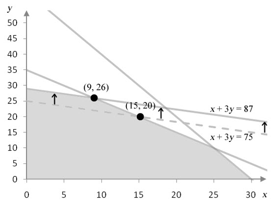
Figure 2 – Increasing the number of hours available for cutting shifts the border of the cutting constraint up.
This change moves the corner point at (15, 20) to (9, 26). The corner point matching the optimal solution has moved.
We would expect the optimal solution to change also.
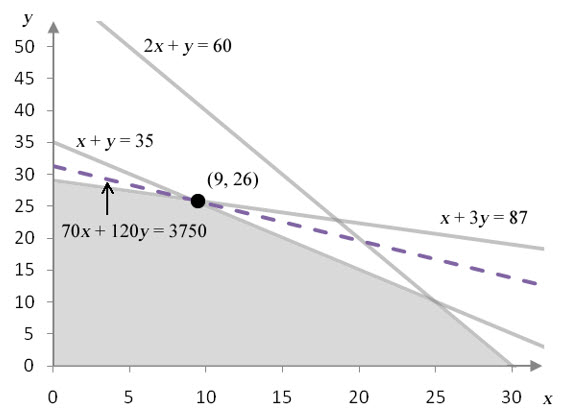
Figure 3 – The solution to the linear programming problem with 87 hours available to cutting.
The corner point matching the optimal solution moves from (15, 20) to (9, 26) when the number of hours for cutting increases by 12 hours. The increased availability of labor increases the profit from $3450 to $3750. The extra 12 hours of labor increases the profit by $300.
We can also see how the profit changes if the number of hours for cutting decreases by 12 hours. In this case, the constraint x + 3y ≤ 75 becomes x + 3y ≤ 63. In this case, the border of the feasible region shifts down.
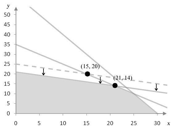
Figure 4 – Decreasing the number of hours available for cutting shifts the border of the cutting constraint down.
This change shifts the corner point from (15, 20) to (21, 14). This ordered pair yields the maximum profit of
P = 70 (21) + 120 (14) = 3150
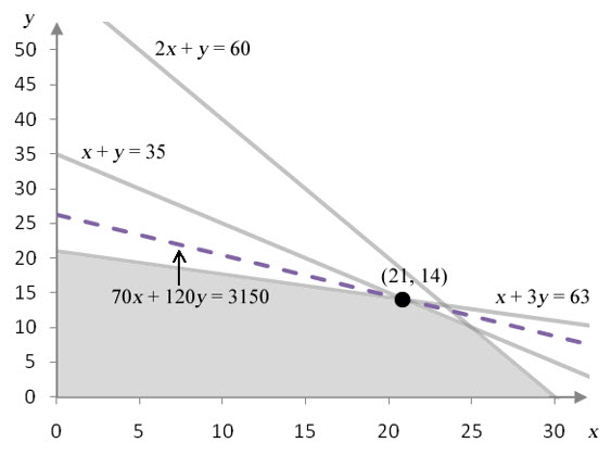
Figure 5 – The solution to the linear programming problem with 63 hours available to cutting.
Decreasing the available cutting time from 75 hours to 63 hours reduces the maximum profit from $3450 to $3150. This tells us that each hour the cutting time is reduced, drops the profit by $25.
Whether the cutting time is increased or decreased by 12 hours, the change in profit is $300. Another way to say this is that a change of one hour of cutting time changes profit by $25 since
This value is called the shadow price of the constraint.
The shadow price of a constraint is the amount the objective function changes at the optimal solution when the constant in the constraint is increased by one unit.
For a standard maximization problem, the shadow price of a constraint appears in the final simplex tableau. Recall the final simplex tableau for this linear programming problem,
The shadow price for the second constraint is located in the fourth column of the indicator row.
Each constraint in the standard maximization problem has a shadow price associated with it. The shadow prices are located in the indicator row of the final simplex tableau beneath the slack variables.
Example 2 Find and Interpret the Shadow Price
The standard linear programming problem from Example 1,
has a final simplex tableau
Suppose amount of material available increased so that an additional 5 frame bags or panniers could be made each week. This will change the first constraint from from x + y ≤ 35 to x + y ≤ 40.
a. Find the shadow price for this constraint.
Solution Increasing the amount of available material for a total of 5 more frame bags and panniers changes the first constraint from x + y ≤ 35 to x + y ≤ 40. The shadow price for this constraint is located in the indicator row under the slack variable corresponding to the constraint, s1. In this case, the shadow price is 45.
b. How will profit change when the total capacity to produce frame bags and panniers is increased from 35 to 40?
Solution The shadow price of 45 relates an increase in the constant in the first constraint to an increase in the objective function. This means increasing the capacity to produce frame bags and panniers by 1 unit increases the profit by $45. A five unit increase would increase the profit by five times as much, 5 ($45) = $225.
Shadow prices help us to make informed decisions about changing the resources (the constants in the constraints) for a problem. Knowing the benefits of changing the constant in one of the constraints allow us to decide whether the costs of making this change is reasonable. For instance, if increasing capacity by five units increases profit by $225, but costs $250 to make that change, then the change is not warranted.
In Example 2, we changed the constant in one of the constraints whose border passed through the optimal solution. Now let’s examine how changing the constant in a constraint whose border does not pass through the optimal solution affects the solution to the linear programming problem. Let’s look the first two constraints at the optimal solution (15, 20):
If the optimal solution is substituted into the left hand side of the first two constraints, the left hand side is equal to the right hand side. This means that at the optimal solution, the entire capacity is being utilized and all of the cutting time is being utilized to produce 15 frame bags and 20 panniers.
This type of behavior defines a binding constraint. At binding constraints, the resources modeled by the constraint are fully utilized.
The same cannot be said of nonbinding constraints. Let’s look at the third constraint at the optimal solution (15, 20):
In this constraint, substituting the optimal solution in the left hand side yields a value of 50. This means that only 50 hours of assembly and finishing time is utilized to produce 15 frame bags and 20 panniers. Ten hours of the available 60 hours for assembly and finishing is not utilized. In the language of linear programming, we say there is 10 hours of slack in this constraint.
If the hours for assembly and finishing are underutilized, adding more time for assembly and finishing will not change the optimal solution.
When the amount of time is for assembly and finishing is decreased by 5 hours, the shape of the feasible region changes. The corner point at (25, 10) moves to (20, 15). At this point, there is still 5 hours of slack, so 5 hours of assembly and finishing time is not being utilized. This has no effect on the optimal solution.
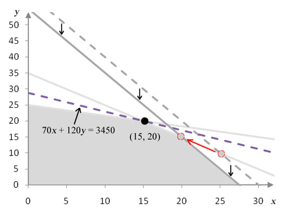
Figure 6 – If the amount of time available for assembly and finishing is reduced by 5 hours to 55 hours, the assembly and finishing constraint shifts down. This moves the corner point at (25,10) to (20, 15).
Once the amount of time is reduced by an amount that eliminates the slack, the constraint on assembly and finishing affects the solution. If the amount of time for assembly and finishing is dropped to 50 hours, all three constraints intersect at the same point, and all three constraints are binding. In this case, the capacity, cutting time and assembly and finishing time are fully utilized.
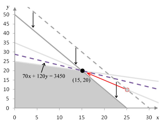
Figure 7 – If the amount of time available for assembly and finishing is reduced by 10 hours to 50 hours, the assembly and finishing constraint shifts down. This moves the corner point at (25,10) to (15, 20).
If the amount of time for assembly and finishing is reduced below 50 hours, the assembly and finishing constraint becomes binding, and the capacity constraint becomes nonbinding. Any changes in the assembly and finishing constraint now move the optimal corner point to a new position.
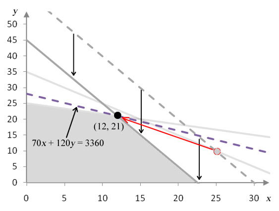
Figure 8 – If the amount of time available for assembly and finishing is reduced by 15 hours to 45 hours, the assembly and finishing constraint shifts down. This reduction causes the optimal solution to change to (12, 20).
For instance, if only 45 hours are available for assembly and finishing, the optimal solution is to produce 12 frame bags and 21 panniers. All of the cutting time and assembly and finishing time is fully utilized, but the capacity is underutilized since only 33 products are being produced.
These changes can be summarized by saying that the total amount of time for assembly and finishing time can be increased above 60 hours an unlimited amount without affecting the optimal solution. But if the total amount of time for assembly and finishing is reduced by more than 10 hours below 50 hours, the optimal solution will move to a new position.
Precautions must be taken when interpreting shadow prices. Shadow prices are valid for the optimal corner point over a range of changes to the constant in a constraint. In the standard maximization problem we have been examining, we can increase the amount of time allotted for cutting by 30 or decrease the amount of time allotted for cutting by 20 and still change the profit 45 for each 1 hour change in cutting time.
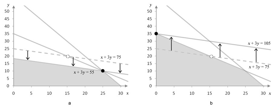
Figure 9 – In graph a, the constant in the second constraint has been decreased from 75 to 55 and the optimal corner point is relocated from (15, 20) to (25, 10). In graph b, the constant in the second constraint has been increased from 75 to 105 and the optimal corner point is relocated from (15, 20) to (0, 35).
As long as the constant on the right hand side of the second constraint varies from 55 to 105, the same two constraints are binding. Any values outside of this range changes which constraints are binding. This occurs because the optimal corner point no longer falls on the border of the cutting constraint and the capacity constraint.
Recall the linear programming problem for the contract breweries from sections 4.2 and 4.4:
In this problem, we wish to minimize the cost C of producing barrels Q1 of American ale from brewery 1 and Q2 barrels of American ale from brewery 2. The final simplex tableau for this problem is
Shadow prices for standard minimization problems are found in a different location of the final simplex tableau. The solution to this problem, (Q1, Q2) = (8000, 2000), is found beneath the slack variables in the indicator row. The shadow prices are located in the first two rows of the last column.
The shadow price for the production requirement is 105. If the production requirement of producing at least 10,000 barrels is increased by 1 unit to 10,001 barrels, the total cost will increase by $105. The shadow price for the constraint -0.25Q1 + Q2 ≥ 0 is 20. If the right hand side were to increase by one unit from 0 to 1, the total cost would increase by $20. Changing the right hand side of Q1 – Q2 ≥ 0 by 1 unit does not change the total cost.