
Suppose we are given some frequencies corresponding to some data in intervals.
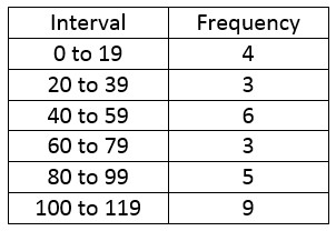
To find the mean, we need to find a representative data value from each interval.
We’ll use the midpoint of each interval. The midpoint for the first interval is
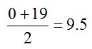
We can find the other midpoints in a similar manner. Let’s add this to the table.
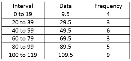
Let’s put this information in a spreadsheet.
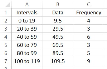
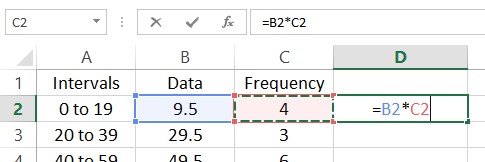
To find the mean of this frequency distribution, multiply each data value times its corresponding frequency. In the spreadsheet, put =B2*C2 in cell D2.
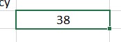
Press Enter to compute this value. Next we need to fill this value into the cells D3 through D7. Click on cell D2. The cell will be outlined like you see below.
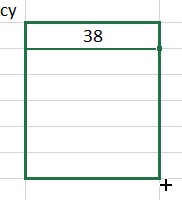
Place your mouse over the box in the lower right hand corner of this outline. The cursor will change to a black cross. Hold down the left mouse button and drag the cursor to cell D7.
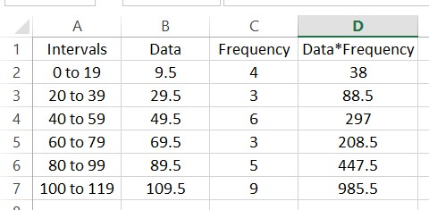
When you release the button, the products will be calculated for each row. Adding a label in cell D1 might help you to remember what the numbers in the cell are.
The function SUM is useful for adding up lists of numbers. For instance, we can find the sum of the frequencies N by typing =SUM(C2:C7). Put this formula in cell B9.
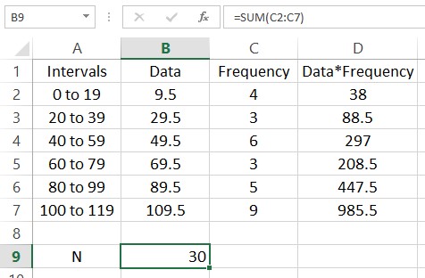
In this picture a label has been added in A9 to help the reader understand what is in the cell to the right. Add another label in cell A10 with the text “Mean”. Next to that cell we’ll calculate the mean of the data. This is done by adding the entries in column D and dividing by the sum of the frequencies in cell B9.

Finding the variance is a bit more complicated. In this calculation we need to subtract the mean from each data value and square the result. This needs to be done with an absolute reference to cell B10 so that the fill always refer to that cell in making the calculation. Start by clicking in cell E2 and typing =B2-$B$10.
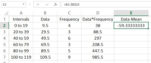
This means that the data value 9.5 is approximately 59.3 units below the mean. Fill the rest of the column and we end up with this worksheet.

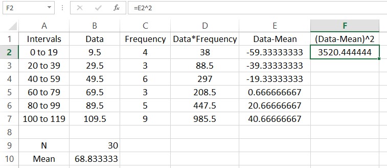
We could sum these deviation now, but the positive and negative nature of each row would mask the spread of the data. Squaring each of the entries makes each of them positive. In cell F2, type =E2^2.
Fill the rest the rows using a fill.
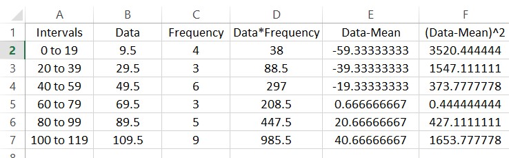
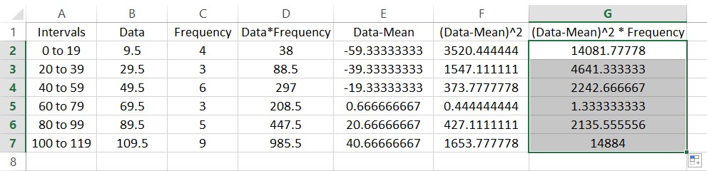
The entries in this column are often called the deviations from the mean squared. Each of these occur with the frequencies in column C. To find the sample variance, multiply the entries in column F by the frequencies in column C to give the worksheet below.
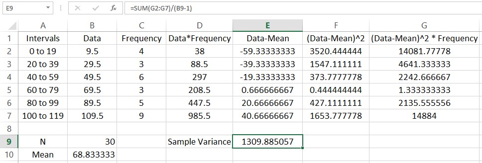
Let’s calculate the variance. Start by typing a label for the sample variance in cell D9. In the adjacent cell we’ll put the value. The variance is the sum of the entries divided by the sum of the frequencies minus 1. In cell E9, type =SUM(G2:G7)/(B9-1).
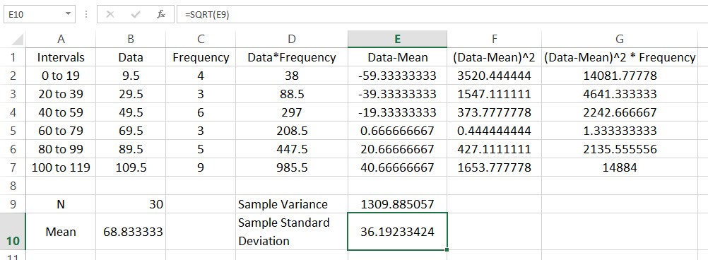
The sample standard deviation is the square root of the standard variance. We can take the square root using the function SQRT. Put a label in cell D10 and type =SQRT(E9) in the adjacent cell.
 The standard deviation is a measure of how spread out the frequency distribution is around the mean.