
How do you graph a system of linear inequalities?
A craft brewery cannot produce unlimited amount of beer each month. As we have seen in this section, there are constraints on the amount of beer that can be fermented as well as the amounts of each ingredient that can be shipped to the brewery and stored on site. If barrels of pale ale and barrels are produced per month,
Together these inequalities define possible combinations that the brewery may produce. In addition, it does not make sense for the amount of beer produced to be negative. So in addition to these inequalities, we also require that
![]() Together these inequalities form a system of linear inequalities.
Together these inequalities form a system of linear inequalities.
A system of linear inequalities is two or more linear inequalities solved simultaneously. Each linear inequality has a solution that is a half plane. The solution set of the system of linear inequalities is all ordered pairs that make all inequalities in the system true. If we examine the solutions sets of each of the individual inequalities together, the solution set of the system of inequalities is where all of the individual solution sets overlap.
The Solution to a System of Linear Inequalities
- Graph the corresponding linear equation for each of the linear inequalities. If the inequality includes an equal sign, graph the equation with a solid line. If the inequality does not include an equals, graph the equation with a dashed line.
- For each inequality, use a test point to determine which side of the line is in the solution set. Instead of using shading to indicate the solution, use arrows along the line pointing in the direction of the solution.
- The solution to the system of linear inequalities is all areas on the graph that are in the solution of all of the inequalities. Shade any areas on the graph that the arrows you drew indicate are in common.
Example 4 Graph the System of Linear Inequalities
Graph the solution set for the system of linear inequalities
Solution To get started, we need to graph the equations y = -2x + 5, x = 0, and y = 0. The first equation will be graphed as a dashed line since the corresponding inequality is a strict inequality. The vertical line x = 0 and horizontal line y = 0 will be graphed as solid lines since the corresponding inequalities include an equal sign.
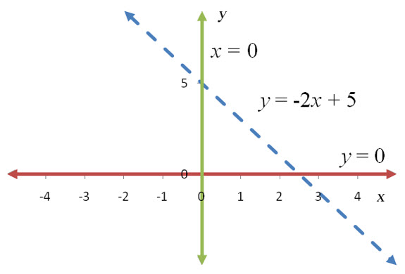
Figure 12 – The corresponding equations for the inequalities in Example 4.
With these boundary lines in place, we need to test a point in each inequality to know the individual solution for each inequality. It is not possible to use (0, 0) since it lies on the horizontal and vertical lines.
Another point that is easy to test is (1, 1).
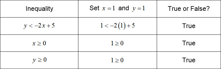
For each line, place arrows on the lines indicating which side is a part of the solution. Since the test point is true in each inequality, we need to place arrows on each line pointing toward the test point.
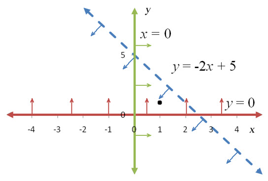
Figure 13 – The arrows on each line point in the direction of the black test point since it makes each inequality true.
Any point in the triangular region where (1,1) lies will make all of the inequalities true. In any other part of the graph, one or two of the inequalities might be true, but not all three in the system. Shade the triangular region where all of the individual solutions overlap to give the graph in Figure 14.
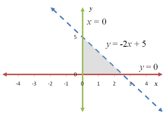
Figure 14 – The solution to the system of linear inequalities. Any ordered pair in the gray shaded region makes all three inequalities true.
When the solution set to a system of inequalities can be enclosed in a circle, the solution is bounded. The solution in Example 4 is an example of a bounded solution set.
Example 5 Graph the System of Linear Inequalities
Graph the solution set for the system of inequalities
Solution In this example, subscripted variables are used. This makes it harder to pick an independent variable. Either variable can be the independent variable. For no particular reason, we’ll graph x1 on the horizontal axis and x2 on the vertical axis.
This system includes the non-negativity constraints x1 > 0 and x2 > 0. These tell us that the solution must lie in a quadrant where all variables are not negative. We can simplify the example by realizing that this is in the first quadrant. By graphing all of the lines primarily in the first quadrant, we can speed up the graphing process.
To graph the other two constraints, we need to graph the lines that form the border of the solution set,
The first equation is in slope-intercept form with a slope of –2/3 and a vertical intercept of 3. Drawing a line through (0, 3) with a slope of –2/3 gives the border of the first constraint.
The second line is easy to graph if we find the intercepts. If we set x1 = 0, we get x2 = 6 yielding the vertical intercept . The other intercept is located by setting x2 =0. The resulting equation can be solved for x1 to yield the horizontal intercept (x1, x2) = (18/5, 0).
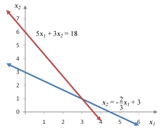
Figure 15 -The borders of the first two inequalities in Example 5. The graph is drawn in the first quadrant due to non-negativity constraints.
Drawing a line through these two ordered pairs results in the border for the second constraint. Both lines must be drawn with a solid line since both constraints include an equal sign in the inequality.
Now pick a test point like (0, 0) to determine which side of each line should be shaded.
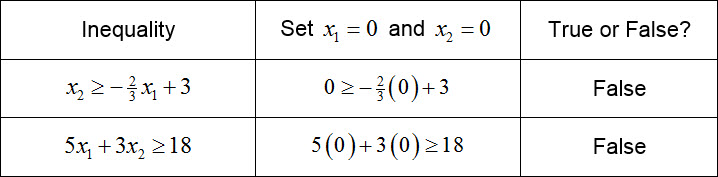
Each inequality is false at the test point so the solution set to each inequality must be on the side of the line where the test point is not located. Use arrows on each line to indicate the side of each line where the test point is not located.
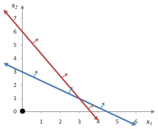
Figure 16 -For each inequality, the side opposite the test point must be shaded since the inequalities are both false at the test point.
The solution set to the system is all of the ordered pairs in the first quadrant (due to the non-negativity constraints) that are solutions to each of the inequalities in the system. By noting where the solution sets for each inequality overlap, we get the solution set below.
Figure 17 – The solution set to the system in Example 5.
Because this solution set extends infinitely far, the region cannot be enclosed in a circle. Solution sets that cannot be enclosed in a circle are called unbounded solution sets.
Example 6 Graph the System of Linear Inequalities
Graph the solution set for the system of inequalities
Solution The border of the solution set is formed by
The first equation is a line in slope-intercept form with a slope of 1 and a vertical intercept of 3. This line is graphed as a solid line since an equal sign is part of the inequality.
The second equation can be solved for y to yield y = x. This is a line with a slope of 1 that passes through the origin. Since the inequality is a strict inequality, the border is graphed with a dashed line.
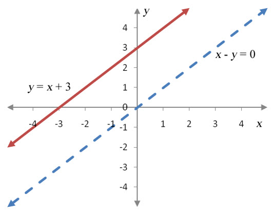
Figure 18 – The borders of the inequalities in Example 6.
The border of the second inequality passes through the ordered pairs (0, 0) and (1, 1), the ordered pairs we have used in other examples as test points. For this example, we’ll use (1, 0) as the test point.
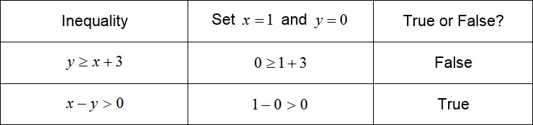
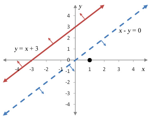
Figure 19 – The borders of the inequalities with arrows indicating the individual inequality solution. The first inequality is false at the test point so the side opposite is the solution. For the second inequality, the inequality is true at the test point so that side is the solution for the inequality.
As with previous examples, the solution set of the system of inequalities is where all of the individual inequality solution sets overlap. Examining the graph carefully, we note that there is no place on the graph where all of the inequalities overlap. There are no ordered pairs that satisfy all of the inequalities simultaneously, so there are no solutions to the system of inequalities.
Now that we’ve tried out the strategy for solving several simple systems of inequalities, let’s revisit the system of inequalities for the craft brewery.
Example 7 Graph the System of Inequalities for the Craft Brewery
The system of inequalities for a craft brewery is
where x1 is the number of barrels of pale ale produced, and x2 is the number of barrels of porter produced. Graph the system of inequalities with as the independent variable.
Solution The non-negativity constraints restrict the solution to the first quadrant. Because of this, we’ll restrict the borders of the other three inequalities to this quadrant and not extend any shading of the final solution beyond the first quadrant.
The borders of the inequalities for capacity, malt, and hops are given by the equations
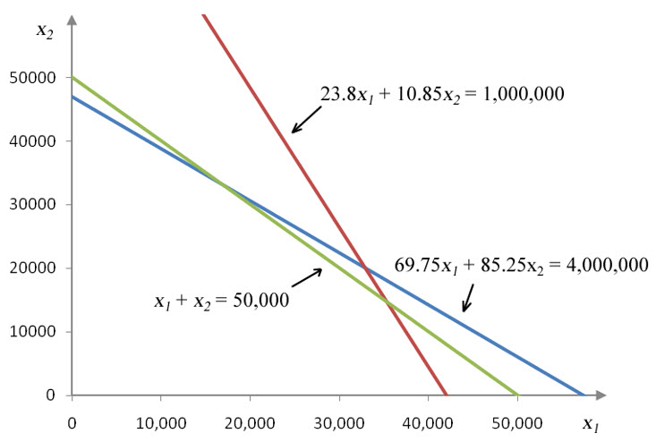
Figure 20 – The borders of the inequalities in Example 7.
Each of these equations was graphed earlier in this section. Putting all of the lines on a single graph yields the graph in Figure 20.
To find the solution sets of each of the inequalities, let’s test the ordered pair (0, 0) in each inequality and indicate shading with arrows in the graph.
Based on this table, the test point must be included in the solution set of each of the inequalities. The arrows on each of the lines must point to the half-plane containing the test point for each inequality.
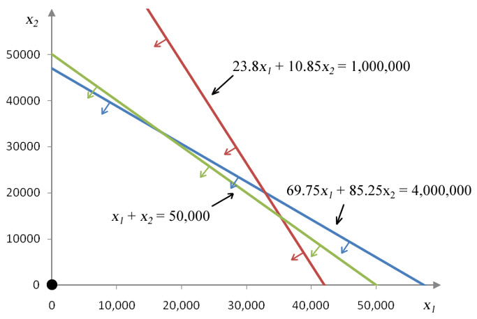
Figure 21 – For each inequality, the test point must be included in the solution suggesting the shading on the graph.
The individual solution sets all overlap in a region that is to the left and below all of the lines.
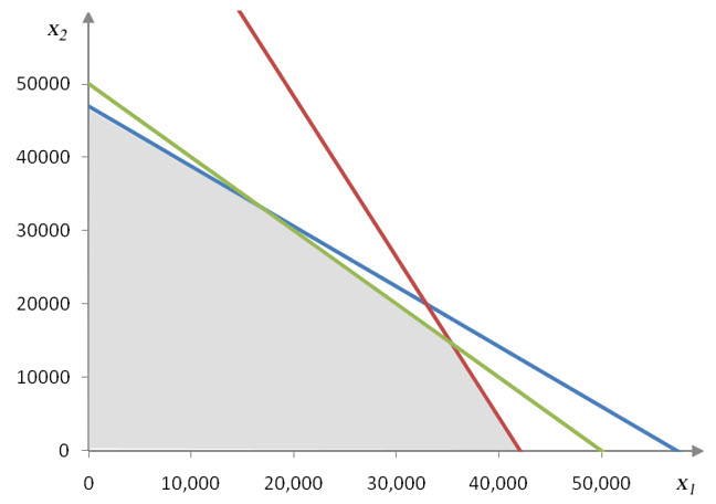
Figure 22 – The region shaded in gray is the solution to the system of inequalities for a craft brewery. This region is where the solutions to all inequalities in the system coincide.
At any point in the solution set, the brewery can produce the number of barrels of beer indicated by the ordered pair and satisfy all of the constraints for capacity, malt and hops.