How do you get the optimal solution to a standard maximization problem with the Simplex Method?
In the previous question, we learned how to make different variables into basic and nonbasic variables. This allowed us to calculate the locations of corner points on the feasible region and other points of intersection. For simple linear programming problems, there can be many such points. If we naively make different variables into basic variables, it may take a very long time to find the corner point that optimizes the objective function.
The Simplex Method is an algorithm for solving standard maximization problems. By following the steps below, you ensure that the points you find by changing basic variables are corner points of the feasible region. In addition, the algorithm is iterative. In other words, it is carried out several times with the result of each iteration providing the starting point to the next iteration. The beauty of the Simplex Method is that each iteration yields a larger value for the objective function and eventually leads to the largest possible value for the objective function.
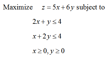
To get a feel for how the Simplex Method works, let’s solve the standard maximization problem
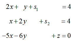
We’ll start by converting this problem to an appropriate system of linear equations. Add a different slack variable to each constraint to yield
To convert the objective function to an appropriate form, move all of the terms with variables to the left side of the equation. This is done by subtracting 5x and 6y from both sides. This yields the equation -5x -6y + z = 0.
These equations form the system of linear equations
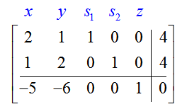
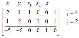
The augmented matrix for this system,
is the initial simplex tableau. It is the starting point for carrying out the Simplex Method algorithm. The bottom row of the tableau is called the indicator row. The algorithm starts by determining which variable will become a basic variable in the first iteration of the algorithm. The variable that corresponds to the most negative entry in the indicator row will become a basic variable.
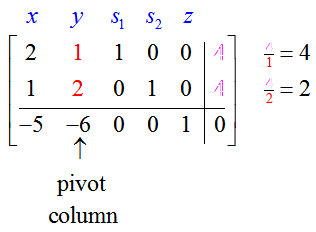
For this matrix, the most negative entry is -6 in the second column. The variable y that corresponds to the column will become the basic variable. This column is the pivot column.
If we pick the column with the most negative entry in the indicator row to be the pivot column, the objective function will increase by the largest amount. Remember, those negative entries correspond to positive coefficients in the original objective function. For the objective function z = 5x + 6y, the most negative entry in the indicator row, -6, corresponds to the largest positive coefficient, 6, in the objective function. Increasing the value of y in the potential solution from 0 to some positive value leads to a larger increase in the objective function value z than increasing the value of x from 0 to the same positive value. This is due to the fact that the coefficient on y is larger than the coefficient of x. In effect, it is more efficient to change y values than x values in the solution.
We know that we’ll need to make all of the entries but one in that column equal to zero via row operations. The other entry will be a one. The row where we will put the one is called the pivot row, and the entry that becomes a one is called the pivot. To find which row will become the pivot row, we form quotients from the entries in the pivot column and the last column:
The row whose quotient is positive and smallest is the pivot row. In this case, the second row is the pivot row so the pivot is the number 2 in this row.
As we saw earlier, picking the pivot row carefully guarantees that the potential solution stays in the feasible region and all variables are non-negative. The variables must remain non-negative for a standard linear programming problem.
Let’s look at this idea more closely. Look at the initial tableau from the standard linear programming problem:
We already know that y will become a basic variable based on the numbers in the indicator row. By making y a basic variable, either s1 or s2 will join x as a nonbasic variable. The question is, which will it be?
Suppose that s1 and x will be the nonbasic variables in the next tableau, and will be set equal to zero. In this case, we can use the first row of the tableau to determine the corresponding value of y:
The value of s2 is found from the second row of the tableau by setting the nonbasic variables equal to zero and y = 4:
This is not a reasonable solution since the slack variable s2 is negative.
Let’s look at making s2 and x the nonbasic variables. In this case, we can use the second row of the tableau to determine the corresponding value of y:
The value of s1 is found from the first row of the tableau,
All variables in this case are non-negative. Note that the values for y in each case are precisely the quotients we use to choose which row becomes the pivot row. By choosing a value for y that is smaller (the smaller quotient), we get a situation in which all variables are non-negative.
Now that we know that the pivot is the 2 in the second row, second column of
we’ll use row operations to change it to a 1. The rest of the pivot column will be changed to zeros using row operations. This change in basic variables will lead to the largest increase in the value of the objective function and keep all variables non-negative.
As shown in Question 3, change the pivot to a one by multiplying the second row by 1/2:
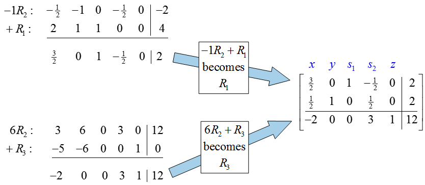
Once the pivot is in place, use row operations to place zeros in the rest of the column:
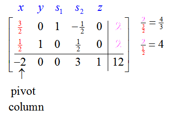
In the Simplex Method, the optimal solution is obtained when there are no negative numbers in the indicator row.
Since the transformed matrix has a negative number in the indicator row, the solution (x, y) = (0, 2) is not optimal. The value of the objective function, z = 12, can be made greater by picking the first column to be the pivot column. To find the pivot row, examine the quotients formed from dividing entries in the last column by corresponding entries in the pivot column:
The smallest quotient is 4/3 in the first row. The pivot, 3/2, is in the first row, first column. As in the first iteration, we must use row operations to change the pivot to a one and change the rest of the pivot column to zeros.
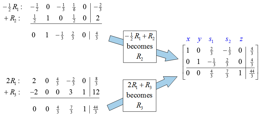
To change the pivot to a one, multiply the first row by 2/3:
To complete the transformation of the pivot column, we must use row operations to put zeros in the rest of the pivot column:
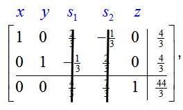
For this tableau, the basic variables are x, y, and z. The nonbasic variables are s1 and s2. The indicator row has no negative entries so this tableau is the final tableau. The optimal solution is read from this tableau by setting the nonbasic variables equal to zero.
If we cover the nonbasic variables,
we see that this tableau corresponds to (x, y) = (4/3, 4/3) and an optimal value of z = 44/3. This is the same value we found graphically in Section 4.2
The process outlined here is summarized in the steps shown here.
The Simplex Method
1. Make sure the linear programming problem is a standard maximization problem.
2. Convert each inequality to an equality by adding a slack variable. Each inequality must have a different slack variable. Each constraint will now be an equality of the form
b1 x1 + b2 x2 + … + bn xn + s = c
where s is the slack variable for the constraint. If more than one slack variable is needed, use subscripts like s1, s2, …
3. Rewrite the objective function z = a1 x1 + a2 x2 + … + an xn by moving all of the variables to the left side. After rewriting the equation, the function will have the form
–a1 x1 – a2 x2 – … – an xn + z = 0
4. Convert the equations from steps 2 and 3 to an initial simplex tableau. Put the equation from step 3 in the bottom row of the tableau and all other equations above it. The bottom row is called the indicator row.
5. Find the entry in the indicator row that is most negative. If two of the entries are most negative and equal, pick the entry that is farthest to the left. The column with this entry is called the pivot column.
6. For each row except the last row, divide the entry in the last column by the entry in the pivot column. The row with the smallest non-negative quotient is the pivot row. If more than one row has the same smallest quotient, the higher of the rows is the pivot row.
7. The pivot is the entry where the pivot row and pivot column intersect. Multiply the pivot row by the reciprocal of the pivot to change it to a 1.
8. To change the rest of the pivot column to zeros, multiply the pivot row by constants and add them to the other rows in the tableau. Replace those rows with the appropriate sums. When complete, the pivot should be a one, and the rest of the pivot column should be zeros.
9. If the indicator does not contain any negative entries, this tableau corresponds to the optimum solution. In this case, cover the nonbasic variables (set the nonbasic variables equal to zero), and read off the solution for the basic variables. Otherwise, repeat steps 5 through 9 until the indicator row contains no negative numbers.
The Simplex Method will reach an optimal solution for a standard maximization problem with any number of variables and any number of inequalities. However, problems with large numbers of variables and inequalities may require many iterations of steps 5 through 9 to reach the optimal solution. Take special care to avoid arithmetic errors when carrying out the row operations. A graphing calculator or spreadsheet can make the task of carrying out the row operations fairly painless.
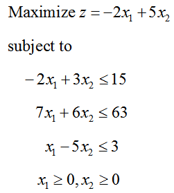
Example 3 Find the Optimal Solution
Find the optimal solution to the linear programming problem
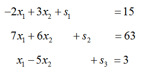
Solution Although this example has three constraints (in addition to the non-negativity constraints), it still has two decision variables. Each constraint needs a slack variable to convert it to an equation. Using the slack variables s1, s2, and s3, the constraints become
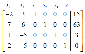
Move all of the variable terms in the objective function to the left side of the equation to yield
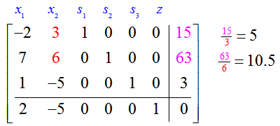
These equations become the initial simplex tableau
The bottom row of the initial simplex tableau is the indicator row. The most negative entry of the indicator row is -5. This means the pivot column is the second column in the tableau.
To determine the pivot row, compute the quotients formed by dividing entries in the last column by entries in the pivot column,
Any negative quotients, such as –3/5 in the third row, are discarded. The quotient formed in the first row, 15/3, is the smallest quotient so the pivot is the 3 in the first row, second column.
In the first iteration of the simplex method, we must use row operations to change the pivot to a one and all other entries in the pivot column to zero.
The pivot is changed to a 1 by multiplying the first row by 1/3. Carrying out the row operation yields
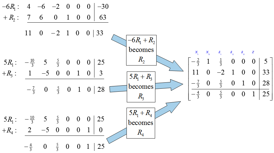
Three row operations are necessary to put the zeros in the rest of the pivot column:
The new tableau corresponds to the solution (x1, x2) = 0, 5) and is not optimal since there is a negative entry in the indicator row.
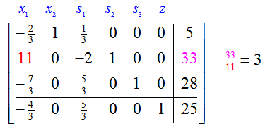
The new pivot column is the first column due to the negative number in the indicator row. To find the new pivot row, compute the quotient formed from dividing the entries in the last column by the entries in the new pivot column:
The second row is the only row with a valid quotient so it is the pivot row. The pivot is the 11 in the second row, first column of the tableau.
Multiply the pivot row by 1/11 to change the pivot to a 1:
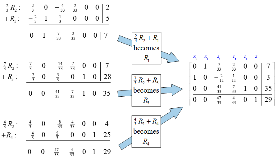
To complete this Simplex Method iteration, we must place zero above and below the pivot using row operations.
Three row operations are required to place the zeros above and below the pivot.
The indicator row does not contain any negative numbers so the optimal solution has been reached.
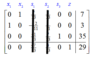
The solution to the linear programming problem is easily observed by covering the columns corresponding to the nonbasic variables s1 and s2:
The optimal solution to the linear programming problem is z = 29 and occurs at (x1, x2) = (3, 7).
