
Any function is graphed with a few basic steps.
- Put the function into the calculator.
- Set the graphing window.
- Graph the function.
The exact sequence of steps is demonstrated in the handout below.
Any function is graphed with a few basic steps.
The exact sequence of steps is demonstrated in the handout below.
Finding a linear model when the data does not follow a perfectly straight line may be referred to by several terms. The terms “method of least squares”, “linear regression”, or “best fit” are all used to refer to modeling data with lines.
We can also use WolframAlpha to model data with lines. To do this we type “linear fit” followed by the data listed as ordered pairs. Here is an example.

You get a graph, the model, and R squared values when you execute this command.
A matrix is entered between curly brackets in WolframAlpha (http://www.wolframalpha.com). Additionally, each row of the matrix is entered in curly brackets too.
You can also put a matrix in reduced row echelon form. We could put the augmented matrix
$latex \displaystyle \left[ \begin{array}{*{35}{l}}
1 & 2 & -1 \\
4 & 3 & 1 \\
\end{array} \right]$
Use the text “row reduce” and then enter the matrix. The solution is x = 1 and y = -1.
Let’s try this with another system of linear equations
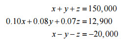
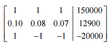
Convert this system into a 3 x 4 augmented matrix:
WolframAlpha understands several commands for putting an augmented matrix into reduced row echelon form. You can use the command rref { }or the command row reduce { }. The matrix goes inside the curly brackets. However, the matrix must be put in carefully. Each row needs to be typed in inside of curly brackets with the entries separated by a commas. In this case, you would type
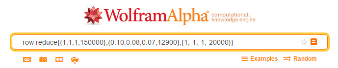
on the command line in WolframAlpha.
After you press Enter, the reduced row echelon form is computed,
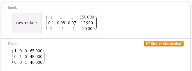
This indicates that the solution to the system is
x = 65,000, y = 45,000, z = 40,000.
To solve a system of linear equations in two variables by graphing, you must first solve each equation for the dependent variable. Once this is done, we can use the equations to find an appropriate window for the graph. It is often useful to also solve the system algebraically…this helps us to establish the horizontal extent of the window.
Problem The annual number of cars produced t years after 2000 by a small car manufacturer is $latex y=6.032t+34.543$ thousand cars. A larger producer has annual production $latex y=-10.564t+100.340$ thousand cars. In what year will the annual production be equal? What will the production be then?
Solution Examine the two equations. The vertical intercepts are 34.543 and 100.340. From 34.543, the first line rises. From 100.340, the second line decreases. Based on this, we can deduce that a vertical window from 0 to 110 is appropriate. If we solve the system by substitution, we see that the point of intersection should be t = 3.965. This suggests a horizontal window of 0 to 5 or 0 to 10. In this window, we can find the point of intersection at (3.965, 58.460).

The value 3.965 corresponds to a time late in the year 2003. The number of cars produced at that time is 58.460 thousand cars or 58,460 cars. Be careful in rounding the t value. Although t = 3.965 rounds to 4 (the year 2004), this time is in the year 2003. Rounding to the nearest integer would put the point of intersection in the next year…a mistake when the problem asked in what year.
Suppose the given square matrix is called A. To find the inverse of any matrix, we write the matrix in a larger matrix along side an identity matrix of the same size,
$latex \displaystyle \left[ \left. A\, \right|\,I \right]$
Now use row operations to rewrite this matrix so that the identity appears on the left side. The inverse of the original matrix will be on the right side of the transformed matrix,
$latex \displaystyle \left[ \left. I\, \right|\,{{A}^{-1}} \right]$
For instance, suppose we want to find the inverse of
$latex \displaystyle A=\left[ \begin{matrix}
2 & 2 \\
2 & 1 \\
\end{matrix} \right]$
Start with
$latex \displaystyle \left[ \left. \begin{matrix}
2 & 2 \\
2 & 1 \\
\end{matrix}\, \right|\,\begin{matrix}
1 & 0 \\
0 & 1 \\
\end{matrix} \right]$
$latex \displaystyle \frac{1}{2}{{R}_{1}}\to {{R}_{1}}$
$latex \displaystyle \left[ \left. \begin{matrix}
1 & 1 \\
2 & 1 \\
\end{matrix} \right|\begin{matrix}
\frac{1}{2} & 0 \\
0 & 1 \\
\end{matrix} \right]$
$latex \displaystyle -2{{R}_{1}}+{{R}_{2}}\to {{R}_{2}}$
$latex \displaystyle \left[ \left. \begin{matrix}
1 & 1 \\
0 & -1 \\
\end{matrix} \right|\begin{matrix}
\frac{1}{2} & 0 \\
-1 & 1 \\
\end{matrix} \right]$
$latex \displaystyle -1{{R}_{2}}\to {{R}_{2}}$
$latex \displaystyle \left[ \left. \begin{matrix}
1 & 1 \\
0 & 1 \\
\end{matrix} \right|\begin{matrix}
\frac{1}{2} & 0 \\
1 & -1 \\
\end{matrix} \right]$
$latex \displaystyle -1{{R}_{2}}+{{R}_{1}}\to {{R}_{1}}$
$latex \displaystyle \left[ \left. \begin{matrix}
1 & 0 \\
0 & 1 \\
\end{matrix} \right|\begin{matrix}
-\frac{1}{2} & 1 \\
1 & -1 \\
\end{matrix} \right]$
Let’s apply this strategy to finding a few more inverses.
Problem 1 Find the inverse of
$latex \displaystyle \left[ \begin{matrix}
2 & 4 \\
2 & 5 \\
\end{matrix} \right]$


Problem 2 Find the inverse of
$latex \displaystyle \left[ \begin{matrix}
1 & 3 \\
2 & 7 \\
\end{matrix} \right]$
