Category: Finite Mathematics Ebook

How do you solve a linear programming problem with a graph?

Now that we have several linear programming problems, let’s look at how we can solve them using the graph of the system of inequalities. The linear programming problem for the craft brewery was found to be

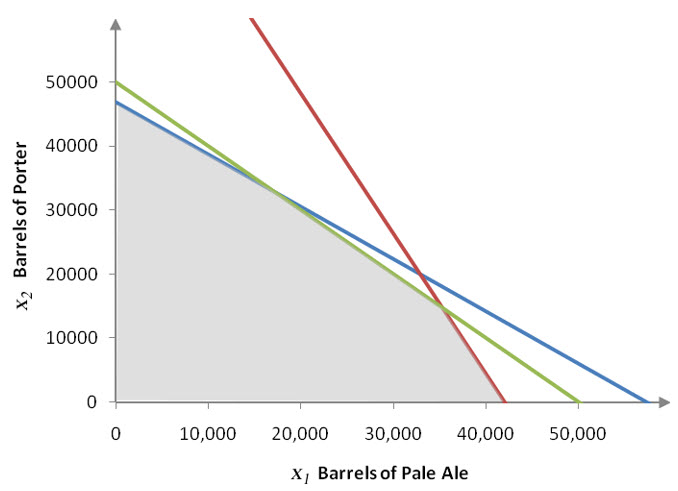
Figure 2 – The feasible region for the craft brewery problem.

The shaded region corresponds to all of the possible combinations of pale ale and porter that satisfy the constraints. Since the solution to the maximization of profit must come from this region, it is called the feasible region. This means that the ordered pairs in the shaded region are feasible solutions for the linear programming problem.

To solve the linear programming problem, we need to find which combination of x₁ and x₂ lead to the greatest profit. We could pick possible combination from the graph and calculate the profit at each location on the graph, but this would be extremely time consuming. Instead we’ll pick a value for the profit and find all of the ordered pairs on the graph that match that profit.

Suppose we start with a profit of $3,000,000. Substitute this value into the objective function to yield the equation

3,000,000 = 100x₁ + 80x₂

If we graph this line on the same graph as the system of inequalities, we get the dashed line labeled P = 3,000,000. A line on which the profit is constant is called an isoprofit line. The prefix iso- means same so that an isoprofit line has the same profit along it. Along the isoprofit line P = 3,000,000, every combination of pale ale and porter leads to a profit of $3,000,000.

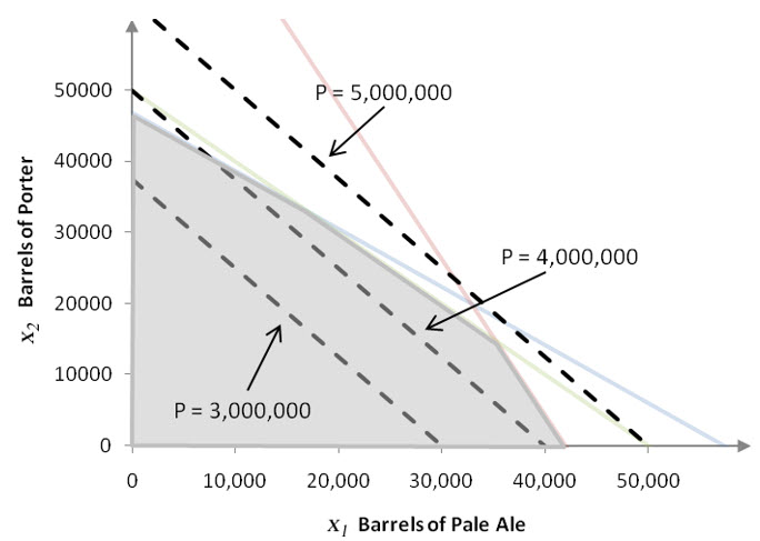
Figure 3 – Several levels of profit at $3,000,000, $4,000,000 and $5,000,000.

The isoprofit lines P = 4,000,000 and P = 5,000,000 can be graphed in the same manner and are pictured in Figure 3.

As profit increases, the isoprofit lines move farther to the right. Higher profit levels lead to similar lines that are farther and farther from the origin. Eventually the isoprofit line is outside of the feasible region. For equally spaced profit levels we get equally spaced parallel lines on the graph. Notice that P = 5,000,000 is completely outside the shaded region. This means that no combination of pale ale and porter will satisfy the inequalities and earn a profit of $5,000,000. There is an isoprofit line, P ≈ 4,706,564, that will just graze the feasible region. This isoprofit line will touch where the border for the capacity constraint and the border of the hops constraint intersect. Points where the borders for the constraints cross are called corner points of the feasible region.

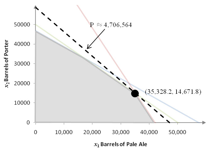
Figure 4 -The optimal production level for the craft brewery rounded to one decimal place. The isoprofit for this level is also graphed.

If the profit is any higher than this level, the isoprofit line no longer contains any ordered pairs from the feasible region. This means that this profit level is the maximum profit and it occurs at the corner point where 35,328.2 barrels of pale ale and 14,671.8 barrels of porter are produced.

Two of the constraint borders intersect at the corner point corresponding to the optimal solution. These constraints, the constraints for capacity and hops, are said to be binding constraints. The malt constraint does not intersect the corner point that maximizes profit so it is a nonbinding constraint.

For resources corresponding to binding constraints, all of the resources are used. In this case, all of the capacity and hops are used to produce the optimal amounts of beer. However, all of the malt is not used which is why the malt constraint is not binding at the optimal solution.

The fact that the optimal solution occurs at a corner point of the feasible region suggests the following insight.

 

We can use this insight to develop the following strategy for solving linear programming problems with two decision variables.

 

By examining the value of the objective function, we can find the maximum or minimum values. If the feasible region is bounded, the maximum and minimum values of the objective function will occur at one or more of the corner points. If two adjacent corner points lead to same maximum (or minimum) value, then the maximum (or minimum) value also occurs at all points on the line connecting the adjacent corner points.

Unbounded feasible regions may or may not have optimal values. However, if the feasible region is in the first quadrant and the coefficients of the objective function are positive, then there is a minimum value at one or more of the corner points. There is no maximum value in this situation. Like a bounded region, if the minimum occurs at two adjacent corner points, it also occurs on the line connecting the adjacent corner points.

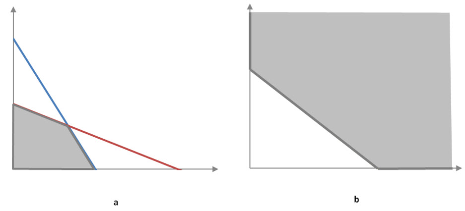
Figure 5 – The feasible region in Graph (a) can be enclosed in a circle so it is a bounded feasible region. The feasible region in Graph (b) extends infinitely far to the upper right so it cannot be enclosed in a circle. This feasible region is unbounded.

Example 2      Solve the Linear Programming Problem Graphically

Solve the linear programming problem graphically:

Solution The feasible region is in the first quadrant since the non-negativity constraints and are included in the system of inequalities.

The other two inequalities are converted to equations and graphed using the horizontal and vertical intercepts.

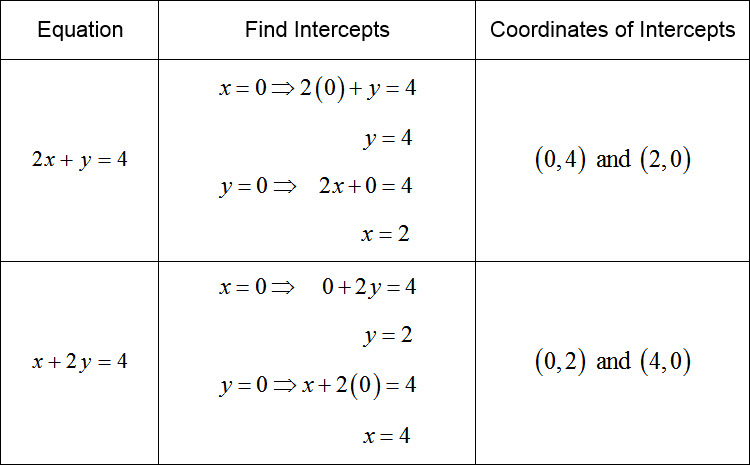
We can graph these intercepts in the first quadrant and connect them with solid lines to yield the following graph.

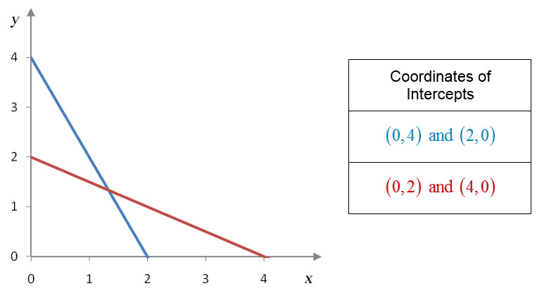
Figure 6 – The borders for the feasible region in Example 2. Since the inequalities are not strict inequalities, the borders are drawn with solid lines.

To determine what portion of this graph corresponds to the feasible region, we need to test the original inequalities with a point from the graph. Although we could choose any ordered pair that is not on one of the lines, in this example we’ll test with (1, 1).

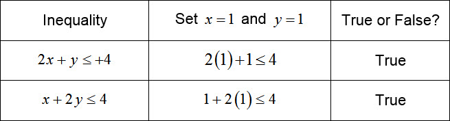
The test point is in the solution set of each inequality. Sketch arrows on each line pointing in the direction of the test point.

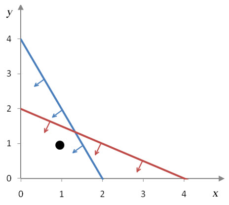
Figure 7 – Since both inequalities are true, the arrows on each line should point in the direction of the test point.

The solution sets for the inequalities overlap in the lower left hand corner of the graph.

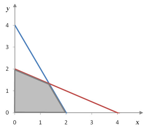
Figure 8 – The feasible region for the linear programming problem in Example 2.

The optimal solution for the linear programming problem must come from this region. Since this is a bounded feasible region, the maximum will occur at one of the corner points. From the graph and the intercepts of the borders, we can see easily identify three corner points: (0, 0), (2, 0), and (0, 2). One more corner point is located at the intersection of the line 2x + y = 4 and x + 2y = 4. We could find this corner point by the Substitution Method, Elimination Method or with matrices, In this example we’ll use the Substitution Method since it is easy to solve for a variable in one of the equations.

To apply the Substitution Method to the system of equations

solve the first equation for y. If we subtract 2x form both sides of the first equation we get y = -2x + 4.

Replace y with -2x + 4 in the second equation and solve for x,

To find y, substitute the value for x into y = -2x + 4 to yield

The solution to the system is x = ⁴/₃ and y = ⁴/₃.

Let’s label the corner points on the graph and calculate the value of the objective function at each of them.

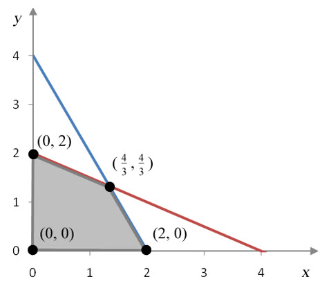
Figure 9 – The feasible region with the corner points labeled.

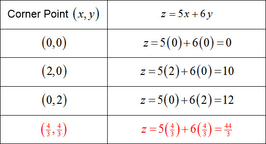
Since ⁴⁴/₃ is approximately 14.67, the corner point at (⁴/₃, ⁴/₃) yields the maximum value of the objective function.

---

Example 3      Solve the Linear Programming Problem Graphically

Solve the linear programming problem graphically:

Solution To graph the system of inequalities, we need to pick an independent variable to graph on the horizontal axis. Although the choice is arbitrary, in this example we’ll graph y₁ on the horizontal axis and y₂ on the vertical axis.

This linear programming problem includes non-negativity constraints, y₁ ≥ 0 and y₂ ≥ 0. In the graph, we’ll account for these constraints by graphing the system of inequalities in the first quadrant only.

The borders for the other two constraints are graphed by utilizing the slope-intercept form of a line and intercepts.

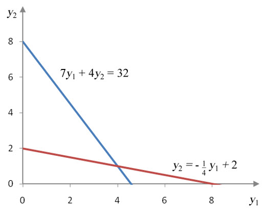
Figure 10 – The borders of the first two constraints in the linear programming problem in Example 3. The graph is shown in the first quadrant due to non-negativity constraints.

Notice that the borders are drawn with solid lines since the inequalities are not strict inequalities. To shade the solution on the graph, substitute the test point (0, 0) into each inequality.

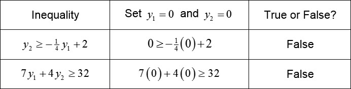
Since each inequality is false, draw arrows on each line pointing away from the test point.

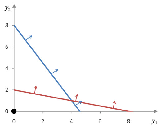
Figure 11 – Since each inequality is false at (0, 0), the side opposite each test point must be shaded.

The shading for each inequality coincides in the upper right portion of the graph.

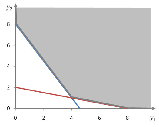
Figure 12 – The feasible region for the system of inequalities for Example 3.

The feasible region extend infinitely far towards the upper right. This feasible region is unbounded since it cannot be enclosed in a circle. A minimum value may or may not exist.

Three corner points are evident in the feasible region. Two of the corner points, (0, 8) and (8, 0), are on the lines drawn earlier. The third corner point occurs where the line y₂ = –¹/₄ y₁ + 2 and the line 7y₁ + 4y₂ = 32 cross.

Figure 13 – The corner points for the feasible region.

Since the first equation, y₂ = –¹/₄ y₁ + 2, is solved for y₂, it is easiest to use the Substitution Method to solve for the intersection point.

Substitute y₂ = –¹/₄ y₁ + 2 into to 7y₁ + 4y₂ = 32 yield

Solve this equation by isolating y₁:

Put this value into the first equation to give y₂ = –¹/₄ (4) + 2 = 1. So the third corner point is located at (y₁, y₂) = (4, 1).

To find the minimum value of the objective function w = 4y₁ + y₂, substitute the corner points.

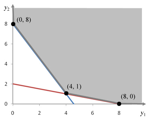
Figure 14 – The feasible region with the corner points labeled.

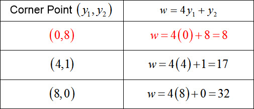
It appears that the minimum is at the ordered pair (y₁, y₂) = (0, 8).

To confirm that the minimum is located at (0, 8), look at three isolevels of w = 4, w = 8, and w = 12. The level should pass through the corner point, but where do the other levels lie?

If we set w equal to each of these levels in the objective function and add these to the graphs, we see how the isolevels behave near the feasible region.

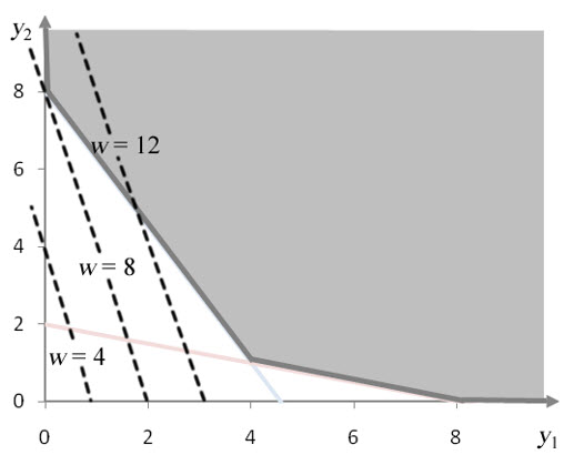
As anticipated, the w = 8 level passes through the corner point at (0, 8). Higher w levels, like w = 12, pass through the feasible region. As w increases, the isolevel lines move farther and farther into the feasible region meaning the feasible region has no maximum value.

We are interested in a minimum value for the objective function. The lowest value of w that includes any points in the feasible region is w = 8. Any levels lower than w = 8, like w = 4, lie completely outside of the feasible region. The level w = 8 passes through the corner point (0, 8) and is the optimal value for the linear programming problem.

---

 

In each of the previous examples, there was one optimal solution. In the next example, there are many possible solutions to the linear programming problem. Each solution yields the same value of the objective function.

Example 4      Solve the Linear Programming Problem Graphically

Solve the linear programming problem graphically:

Solution As with the earlier examples, the non-negativity constraints allow us to graph the system of inequalities in the first quadrant only. To graph the borders of the other three constraints, convert each of the inequalities to equations,

The line x = 8 is a vertical line passing through the horizontal axis at (8, 0). We can place these three lines on a graph as shown in Figure 15.

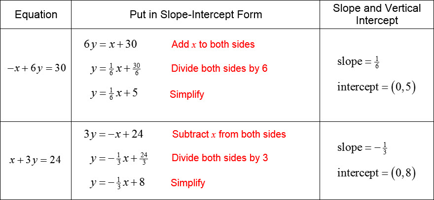
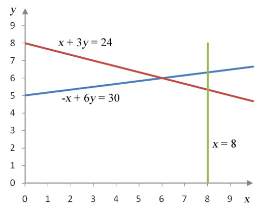
Figure 15 – A graph of the border of each inequality in Example 4.

To shade the solution on the graph, substitute the test point into each inequality.

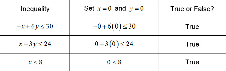
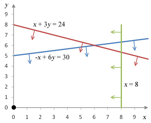
Figure 16 – Since each inequality is true, shade the half plane formed by each inequality where the test point lies.

The individual solution sets all overlap in the feasible region shown below.

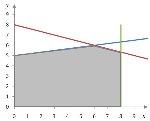
Figure 17 – The feasible region for the system of inequalities in Example 4.

Since this feasible region is bounded, the maximum value of the objective function is located at one of the corner points or along a line connecting adjacent corner points.Several of the corner points are easily identified from the intercepts. However, the two corner points in the upper-right corner of the feasible region are not so obvious.

The red border, given by the line x + 3y = 24, and the green line, given by x = 8, intersect at one of these corner points.

If we substitute x = 8 into x + 3y = 24, we can solve for y to get the first corner point:

The corner point is at (8, ¹⁶/₃).

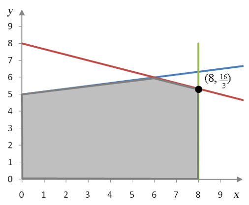
Figure 18 – The feasible region with a corner point shown.

Another corner point is where red line, x + 3y = 24, intersects the blue line, –x + 6y = 30. Using the Substitution Method, we can solve for x in the first equation to yield x = -3y + 24. Substitute the expression -3y + 24 for x in the second equation and solve for y:

If we set y = 6 in x = -3y + 24, we get the corresponding x value, x = 6.

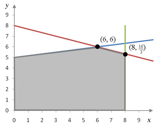
Figure 19 – The feasible region with a corner points at (6, 6) and shown (8, ¹⁶/₃).

Now that we have the corner points, we can substitute the coordinates into the objective function to find the maximum value.

 

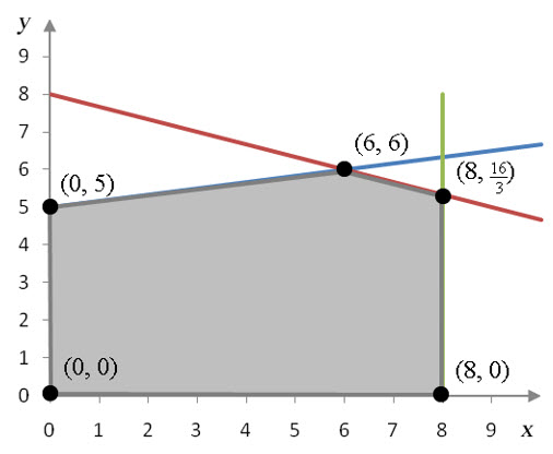
Figure 20 – The corner points and the corresponding values of the objective function.

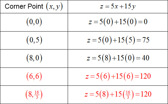
Two adjacent corner points yield the same value, z = 120. This means that the objective function is maximized at any point of a line connecting (6, 6) and (8, ¹⁶/₃).

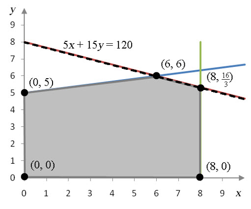
Figure 21 – The isolevel z = 120 passes through two adjacent corner points indicating that the objective function is optimized anywhere on the line connecting the points.

If we graph the isolevel 5x + 15y = 120 on the feasible region, we see that it passes through these points.

For any higher isolevel, the line would be outside of the feasible region. Therefore, this level is the maximum value of the objective function.

What is a linear programming problem?

Linear programming is a strategy for maximizing or minimizing a linear function of several variables. This function is called the objective function and takes the form

z = a₁ x₁ + a₂ x₂ + …+ a_n x_n

Although this equation may look imposing, we can break it down into a simple pattern. Each term on the right hand side consists of a constant called a_n multiplied by a decision variable x_n. The names of the constants and variables are irrelevant, but the constant a_n always multiplies the decision variable x_n raised to the first power. The decision variables are the variables that represent the quantities that may be varied. The variable z represents the quantity being maximized or minimized.

A linear programming problem consists of an objective function and a system of inequalities that defines acceptable values for the variables x₁ through x_n.

 

In a linear programming problem, the constants a₁,…,a_n, b₁,…,b_n and c are real numbers.

The values of the decision variables that optimize (maximize or minimize) the value of the objective function are called the optimal solution of the linear programming problem.

Businesses typically try to either maximize profit or minimize cost by varying the values of the decision variables. With the addition of an objective function, the craft brewery problem can be written as a linear programming problem. Suppose that each barrel of pale ale yields $100 of profit and each barrel of porter yields $80 of profit. We can multiply the profit per barrel times the number of barrels for each type of beer to get the profit for each type of beer. The profit from barrels x₁ of pale ale is

and the profit from x₂ barrels of porter is

The total profit P is the sum of the profit from each type of beer,

P = 100 x₁ + 80 x₂

Although this equation does not utilize z as a variable, it is the objective function for a craft brewery. The names of the variables are not important. We could just as easily used z instead of P or Q₁ and Q₂ instead of x₁ and x₂. The key ingredient of a linear objective function is that the decision variables are raised to the first power, multiplied by a constant and then added together.

With this objective function in hand, we can write out the linear programming problem for the craft brewery:

In the next question, we’ll examine how this problem can be solved using a graph of the solution of the system of inequalities.

Example 1      Find the Linear Programming Problem

Some breweries contract with other breweries to brew a portion of their annual output. By doing this, they avoid the high fixed costs associated with setting up and operating a brewing facility. One brewery, Patrick Henry Brewing, contracts with two other breweries to produce an American ale. It costs the brewery $100 per barrel to produce the beer at the first contract brewery and $125 per barrel to produce the beer at the second contract brewery. To satisfy orders from distributors, Patrick Henry Brewing must contract for a total of at least 10,000 barrels per month. In addition, the amount that is contracted from the second brewery must be at least 25% of the amount contracted from the first brewery. However, labor agreements require that the amount contracted from the second brewery cannot exceed the amount contracted from the first brewery.

Write out the linear programming problem for determining how many barrels should be produced from each contract brewer to ensure that the total cost is minimized?

Solution To begin, identify what we are trying to find and define variables to reflect the unknowns. Since Patrick Henry Brewing needs to know how many barrels of American ale to produce at each of the contract brewers, define the variables as follows:

Q₁: Number of barrels produced at contract brewery 1

Q₂: Number of barrels produced at contract brewery 2

Producing these quantities costs Patrick Henry Brewing $100 per barrel at brewery 1 and $125 per barrel at brewery 2. The cost to produce Q₁ barrels at contract brewery 1 is

and the cost to produce Q₂ barrels at contract brewery 2 is

The total cost C is the sum of the individual costs from each contract brewery,

C = 100Q₁ + 125Q₂

We want to minimize the total cost subject to any constraints on production.

The inequalities are signaled by phrases like “at least” and “cannot exceed”. First we note that the brewery must contract for at least 10,000 barrels per month. This means that in any month,

The phrase “at least” means that the total amount contracted must be greater than or equal to 10,000. Substituting the sum of the variables for the total amount contracted yields

Q₁ + Q₂ ≥ 10,000

Similarly, the amount contracted from brewery 2 must be at least 25% of the amount contracted from brewery 1 or

Since the amount contracted from the second brewery cannot exceed the amount contracted from the first brewery, we can also write

Q₂ ≤ Q₁

Putting the objective function together with the inequalities (including non-negativity constraints) gives the linear programming problem

The non-negativity constraints are needed since the number of barrels of beer from each contract brewery cannot be negative. We’ll find the solution to this linear programming problem in the next question.

How do you solve a matrix equation using the matrix inverse?

In the previous question, we wrote systems of equations as a matrix equation AX = B. In this format, the matrix A contains the coefficients on the variables, matrix X contains the variables, and matrix B contains the constants. Solving the system of equations means that we need to solve for the variable matrix X. This is accomplished by multiplying both sides of the matrix equation by the inverse of the coefficient matrix, A^-1.

A^-1 AX = A^-1 B

The product of a matrix A and its inverse is the identity matrix I. This means we can simplify the matrix equation to

IX = A^-1 B

The product of an identity matrix I with X is simply X, so the solution to the matrix equation is

X = A^-1 B

Example 3      Solve a Linear System with the Inverse

Solve the system of linear equations using the inverse of the coefficient matrix.

Solution In Example 1, we wrote this system as the matrix equation , where

In section 3.3, we found the inverse of A,

We can use the inverse to compute the solution to the system.

The solution is found by multiplying the inverse of A times the constant matrix B,

Since the individual entries in X correspond to the variables x and y, this tells us that x = -21 and y = 16. We can check these values in the original system to make sure they solve the system:

---

 

Example 4      Solve a Linear System with the Inverse

Solve the system of linear equations with the inverse of the coefficient matrix.

Solution This system of equations is equivalent to the matrix equation AX = B where

The variable matrix may be solved for using the inverse of the coefficient matrix, X = A^-1 B. We found the inverse of this coefficient matrix in Example 5 of section 3.3.

Equating the entries in the variable matrix with the entries in this product, we observe that x = 3, y = 4, and z = 5.

---

 

For systems of linear equations with unique solutions, we can use inverses to solve for the variables. Many of the applications in Chapter 2 may be solved using this strategy.

Example 5      Mixing Ethanol Blends

In Example 12 of section 2.2 we created a system of equations to describe a mix of E10 and E85 ethanol,

where E10 is the amount of 10% ethanol pumped in gallons and E85 is the amount of 85% ethanol pumped in gallons. The first equation describes the total amount in the mixture, 10 gallons. The second equation describes the total amount of ethanol in the mixture, 20% of 10 gallons or 2 gallons.

a. Solve this system of equations by finding the inverse of the coefficient matrix.

Solution This system of equations was solved in Chapter 2 using the Substitution Method. In this section we’ll solve the same system by writing the system as a matrix equation.

We can write this system of equations as the matrix equation AX = B by identifying the matrices,

The solution to the matrix equation is X = A^-1 B and requires the inverse of the matrix A.

We begin the process of finding the inverse of A by placing the coefficient matrix in a new matrix alongside a 2 x 2 identity matrix.

Since the entry in the first row, first column is already a 1, we’ll make the rest of the column into zeros using row operations. To do this, multiply the first row by -0.10 and add it to the second row. Place the sum in the second row:

With the first column transformed, proceed to the second column and use row operations to create a 1 in the second row, second column.

We put a 1 in the second row, second column by multiplying the second row by ¹/_0.75. Since 0.75 = ³/₄, this is the same as multiplying by ⁴/₃:

Now multiply the second row by -1 and add it to the first row. Place the result in the first row:

The inverse matrix is the right hand side of this matrix,

The solution to the original system of equations is

Since the variable matrix X represents , this means that the amount of E10 needed is ²⁶/₃ gallons and the amount of E85 needed is ⁴/₃ gallons.

b. If the number of gallons in the mixture should be 12 gallons, how much 10% ethanol and 85% ethanol must be pumped?

Solution If the total number of gallons in the mixture is increased to 12 gallons, the total amount of ethanol in the mixture is or 2.4 gallons. The system of equations becomes

The only change to the system of equations is in the constants, not the coefficients.

This means that we may use the existing coefficient matrix A and the corresponding inverse A^-1 to find the solution of this system,

The constant matrix for this system is

and the solution is

Since the coefficients in the system have not changed, there is no need to recompute the inverse. We may use the inverse from part a to calculate the product. We must mix ⁵²/₅ gallons of E10 and ⁸/₅ gallons of E85.

---

 

This example illustrated the power of using inverses to solve a system of linear equations. As long as the coefficient matrix does not change, the same inverse may be used to solve several different problems with different constant matrices. The solutions are simply the product of the inverse of the coefficient matrices and the different constants. For part a, the constant was  and for part b the constant was . There was no need to recompute the inverse for the different parts.

How do you write a system of equations as a matrix equation?

In section 3.2, you learned how to multiply two matrices. This process involved multiplying the entries in the row of one matrix by the columns of another matrix and then adding those products. For instance, suppose we multiply

Since we are multiplying a 2 x 2 matrix by a 2 x 1 matrix, the product is a 2 x 1 matrix. Working out the product, we get

When the product is written this way, we can easily identify the product of the numbers in the rows of the first matrix with the numbers in the second matrix as well as the sum.

Instead of multiplying the first matrix by a constant column matrix, let’s try multiplying by a matrix containing two variables x and y,

When we carry out the multiplication now, we get

The entries in the product look a lot like the part of a system of equations. In fact, if we set this equal to a 2 x 1 matrix with constants,

we can write the matrix equation as an equivalent system of equations.

These matrices are equal when the corresponding entries are equal or when

In other words,

When a system of equations is written in terms of matrices, we call it a matrix equation. In this matrix equation, the three matrices are typically called A, X and B.

The matrix A is called the coefficient matrix and it entries are the coefficients on the variables when they are written in the same order in each equation. The matrix X is called the variable matrix and contains the two variables in the problem. The matrix B is called the constant matrix and contains the constants from the right hand side of the matrix equation.

To match the different matrices with their entries, each equation must have the variables on the left side with the variable terms listed in the same order. The constants must be on the right side. Once each equation has this format, we can read the entries in each matrix.

Example 1      Write a Linear System as a Matrix Equation

Write the system of linear equations

as the matrix equation AX = B.

Solution The system is in the proper format to determine the coefficient matrix and the constant matrix. The variable matrix for this system is

Using the coefficients on the variables, define the coefficient matrix and constant matrix as

With these definitions, the product AX is equal to

When this matrix is set equal to the constant matrix B, we get

These matrices are equal when x + y = -5 and 3x + 4y = 1. This means the matrix equation is equivalent to the original system of equations.

---

 

We can use the same strategy to write larger systems of equations as matrix equations. This leads to larger matrices. We incorporate different variable names into the variable matrix X as shown in the next example.

Example 2      Write a Linear System as a Matrix Equation

Write the system of linear equations

as a matrix equation AX = B.

Solution Before we can define the matrices, we need to put each equation in the proper format. In the first and second equations, all variable terms are on one side of the equation and the constant terms are on the other side of the equations. In the third equation, there are variable terms on both sides of the equation. We can put the third equation in the proper format by subtracting from both sides of the equation,

This leads to the system

The variable matrix is

The coefficients on the variables give the coefficient matrix,

Note that any signs are included in the coefficients and variables that are missing correspond to a coefficient of zero.

The constant matrix,

matches the constants on the right hand of the system.

We can check to see that the matrix equation AX = B is equivalent to the system by carrying out the product AX:

If we set this matrix equal to B,

the corresponding entries must be equal. This is equivalent to the original system after it had been modified to put it into the proper format.

---

Once a system of linear equations is written as a matrix equation , we can use the inverse of the matrix A to find the solution to the system. In the next question, we’ll learn how to do this and use it to solve an application.

 

How do you find a matrix inverse?

In the previous question, we learned how to check whether two matrices A and B are inverses of each other by computing their products AB and BA. If the products are both equal to the identity matrix I, the matrices are inverses. This property is useful for checking the matrices, but not helpful for finding the inverse of a matrix in the first place.

To find the inverse of a square matrix, the matrix is combined with an identity matrix of the same size in a single matrix. If the matrix is called A, we write this symbolically as [A | I]. If the matrix A is a 2 x 2 matrix, combining it with a 2 x 2 identity matrix results in a 2 x 4 matrix.

The inverse matrix is found by using row operations to transform the matrix so that the identity matrix is on the left side of the combined matrix. The right side of the matrix is the inverse of the matrix A. Symbolically, we must use row operations to yield [I | A^-1].

Example 4      Find a Matrix Inverse

Find the inverse of the matrix .

Solution Combine the matrix with the 2 x 2 identity matrix to yield

We need to use row operations to move the identity matrix to the left side of this matrix. We’ll work with the first column and then the second column to make this change.

In the first column, we want to use row operations to put a 1 at the top of the column and then place zeros below it. Since the first column already has a 1 in the first row, first column, we simply need to use row operations to put a zero below it.

To put a zero in the second row, first column, multiply the first row by -3 and add it to the second row. Place the sum in place of the second row:

Once the first column of the identity matrix is established on the left half of the matrix, we must use row operations to establish the second column of the identity matrix. The 1 in the second row, second column is already in place.

To put a zero in the first row, second column, multiply the second row by -1 and add it to the first row. Place the sum in the first row.

The left side of the matrix is the 2 x 2 identity matrix so the right side is the inverse matrix. In other words, the inverse of is .

We can check this assertion by multiplying the matrices, in two possible orders, to ensure the products are the 2 x 2 identity matrix.

The procedure in Example 4 is also used to find the inverse of larger square matrices.

 

This strategy may be applied to any size matrix A, but in practice it is rarely applied to any matrix larger than 3 x 3. For these larger matrices, a spreadsheet or graphing calculator is used to find the inverse.

In the next example, let’s find the inverse of a 3 x 3 matrix using the strategy above.

Example 5      Find a Matrix Inverse

Find the inverse of the matrix .

Solution Place the matrix in a new matrix with the 3 x 3 identity matrix to yield

We must use row operations to change the left side of the matrix to the identity matrix, one column at a time. In each column we’ll place a 1 in the appropriate position and then place zeros in the rest of the column.

For the first column, there is already 1 in the first row, first column. This means we can go straight to using row operations to put zeros in the rest of the first column.

To put a zero in the first column, second row, multiply the first row by -2 and add it to the second row. Place the sum in the second row. At the same time we add the first and third rows to put a zero in the first column, third row.

To place a 1 in the second row, second column, without changing the first column, interchange the second and third rows.

To complete the second column, a zero needs to be created in the first row second column. Multiply the second row by -1 and it to the first row. Place this sum in the first row.

The entry in the third row, third column must be changed to a 1 using row operations. Multiply the third row by -1 and place the result in the third row.

Two more row operations are needed to change the third column into the third column of the identity matrix.

The inverse matrix is the 3 x 3 matrix on the right side of this transformed matrix so

---

 

For some matrices, it is not possible to find an inverse. In the next example, we examine one of these matrices. Although the matrix is called B, the strategy is exactly the same as other examples.

Example 6      Find a Matrix Inverse

Find the inverse of the matrix .

Solution Place the matrix B in a new matrix next to a 2 x 2 identity matrix,

To change the entry in the first row, first column to a one, multiply the first row by ¹/₂.

Now add -3 times the first row and add it to the second row. Place the sum in the second row.

In carrying out the row operations to find the inverse, the second row in the left hand side of the matrix becomes zeros,

Because of these zeros, it is not possible to use row operations to change the left hand side of the matrix into the identity matrix. This means that the matrix B does not have an inverse.

---

 

In the next section, we’ll use the inverse of a matrix to solve systems of linear equations.