Section 1.2 Question 2

How do you graph a linear function?

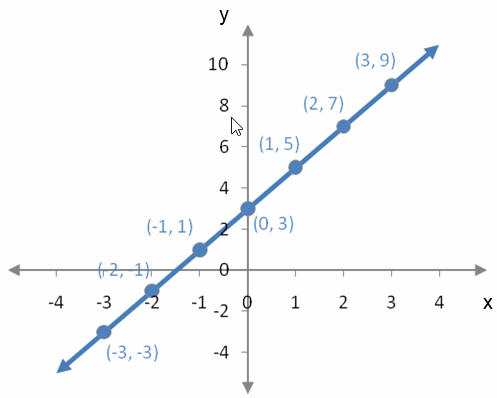
Consider the x value and the y value on an equation y = 2x + 3 as an ordered pair, (x, y). The values can be graphed as shown below.

Figure 1 – The ordered pairs from Table 1and the line passing through the ordered pairs.

Each of the ordered pairs we just found lie along a straight line. This line is related to the constants m and b in the linear function.

For the linear function f (x) = 2x + 3, the value of the constant b is b = 3. This indicates that the function crosses the y axis at the ordered pair (0, 3).

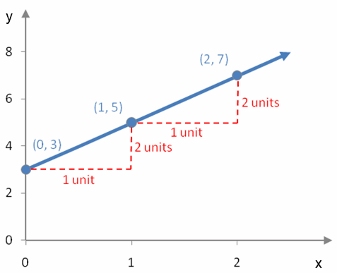
Figure 2 – A closer look at y = 2x + 3 showing the y intercept at (0, 3) and the changes in the variables at ordered pairs along the line.

The constant m in a linear function is related to how the variables change with respect to each other as you move from point to point along the line. In Figure 2, three points are shown on the line. The horizontal change between each ordered pair is 1 unit. The vertical change between each ordered pair is 2 units. The ratio of these changes describes how the variables change with respect to each other and is equal to

This ratio is called the rate of change of the linear function.

When viewed on a graph, this rate is called the slope of the line. Knowing the slope and the vertical intercept of the line corresponding to a linear function allows us to graph the linear function quickly.

Example 1     Graph a Linear Function

For each part below, graph the line corresponding to the linear function.

a.  f (x) = 3x – 1

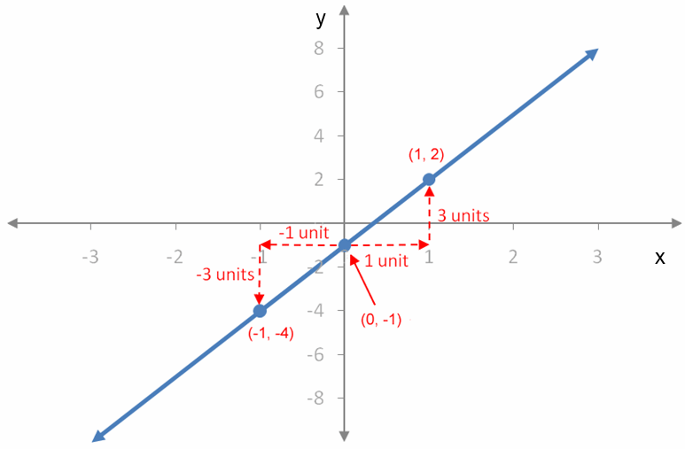
Solution To graph this function, we’ll identify the values of the constants and interpret them to find points on the line. To match the form f (x) = mx + b, rewrite the function as f(x) = 3x + (-1). This tells us that b = -1 and m = 3. Geometrically we know that the vertical intercept is at (0, -1) and the slope is 3. Place a point on the graph at the vertically intercept and then draw a second with respect to that point using

Each of these ratios is equal to 3. We could also use any other ratio equal to 3, but these are the simplest to visualize.

Figure 3 – From the intercept at (0, -1), move either left or right by 1 unit and up or down by 3 units to generate a second point on the line. Once two points are graphed, the graph of the linear function can be drawn through the two points.

b.  g(x) = –¹/₂ x +4

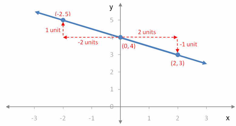
Solution  For this function, b = 4 and m = –¹/₂. This means the vertical intercept is located at (0, 4) and the ratio of vertical change to horizontal change is –¹/₂ or ¹/_-2. Either ratio gives the same slope. The line passing through the corresponding points is graphed in Figure 4.

Figure 4 – By moving left or right 2 units and then up or down 1 unit gives two more points on the line.

c.  h(x) = -2

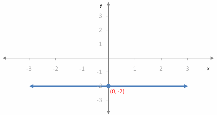
Solution  Write the function in the form h(x) = 0x + (-2). For this function, b = -2 and m = 0. Since the slope is zero, the line must have no vertical change and is a horizontal line.

Figure 5 – A constant linear function is a horizontal line through the vertical intercept.

---

The different parts of Example 1 illustrate the role that the constant m plays on the graph of a linear function. A positive slope leads to a graph that rises as you move from left to right. A graph with this type of behavior is increasing. A negative slope leads to a graph that falls as you move from the left to right. A graph with this type of behavior is decreasing. Graphs with zero slope stay at the same level as you move from left to right on the graph. A graph with this type of behavior is said to be constant.

Figure 6 – Examples of (a) an increasing linear function, (b) a decreasing linear function, and (c) a constant linear function.