
What are demand and supply?
An important application of linear functions is the connection between the price of a good or service and the quantity of a good or service. If we are interested in the relationship between the price and the quantity demanded by consumers at that price, this connection is described by the demand function. The relationship between price of a good or service and the quantity supplied by manufacturers at that price is described by the supply function. These functions describe how consumers and suppliers behave as price is changed.
The consumer’s behavior is given by a table called a demand schedule. This table reflects the relationship between the price of some good or service and the quantity of this good or service demanded at this price. The table below is a typical demand schedule in some market.
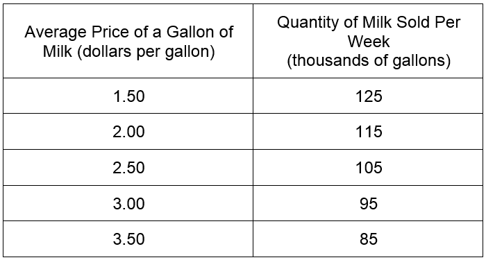
In the first column of the demand schedule are prices of some good. In the other column is the corresponding numbers of that good sold to consumers. From this demand schedule for dairies in a competitive market, we can see that as the price per gallon for milk increases the quantity of milk sold per week decreases. The law of demand states that if everything else is held constant, as the price of the good increases, the quantity demanded drops. This pattern is visible in the demand curve shown below.
The demand function is traditionally graphed with the quantity as the independent variable and the price as the dependent variable. Because of this, quantity is graphed on the horizontal axis and price is graphed on the vertical axis. This means that the information indicating that 125,000 gallons of milk is sold per week at a price of $1.50 per gallon corresponds to the ordered pair (125, 1.50). The demand function takes an input of quantity and outputs price,
P = D(Q)
Demand curves can have many shapes, but the simplest curve is a demand curve follows a straight line. In the case of the demand function for dairies in a market shown here, we’ll find a linear demand function of the form
D(Q) = mQ + b
This is the same form defined earlier, f (x) = mx + b, with the variable changed to Q from x and the name changed to D from f.
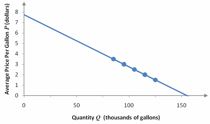
Figure 11 – The demand D(Q) for milk.
Example 6 Find the Demand Function for Milk
Find the equation of the demand curve graphed in Figure 11.
Solution The graph above gives us a hint that the demand function is a linear function. To make sure the ordered pairs all lie along a straight line, we need to find the slope between adjacent ordered pairs.
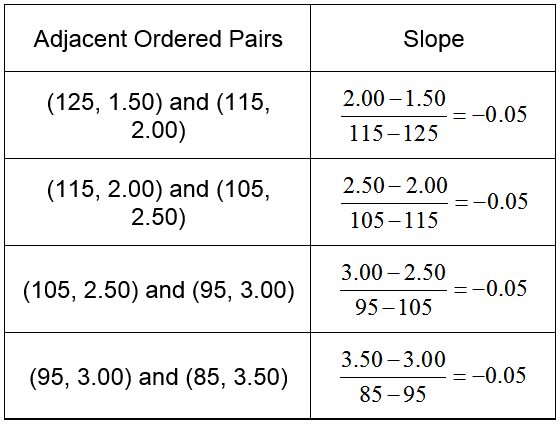
Table 6
Since the slope between any pair of adjacent points is -0.05, all of the points lie along a line with slope -0.05.
Insert the slope into the form for a linear demand function to yield
D(Q) = -0.05Q + b
All that remains is to find the vertical intercept b in the function. None of the points are the vertical intercept. To find b, substitute any of the points into the function. Let’s try the ordered pair (125, 1.50):
D(125) = -0.05 (125) + b = 1.50
To find the value of b, simplify the equation to give
-6.25 + b = 1.50
Adding 6.25 to both sides leads to b equal to 7.75. The function for demand is
D(Q) = -0.05Q + 7.75
The supply function also relates the price of a good or service to a quantity of the good or service. Unlike the demand function which describes the consumer’s willingness and ability to buy a good or service, the supply function describes the willingness and ability of a business to supply a good or service at a given price. If all other factors are held constant, as the price rises the quantity supplied will also increase. A higher price leads to more profit for a business encouraging higher production.
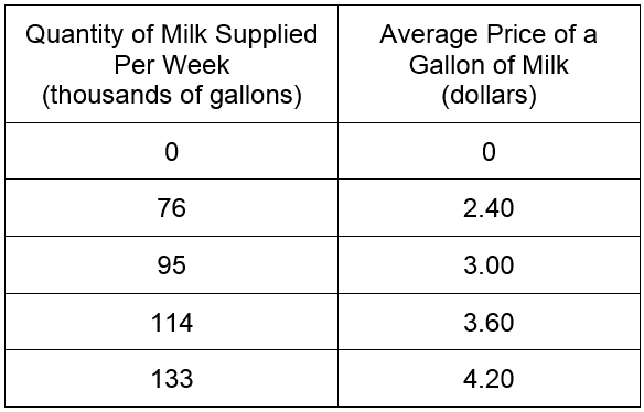
A supply schedule is a table that shows the relationship between the price of a good or service and the quantity supplied by a firm.
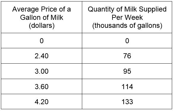
Table 7
In this supply schedule, an increase in the average price of a gallon of milk corresponds to an increase in the quantity of milk supplied by dairies. A graph of the data shows a straight line with a positive slope.
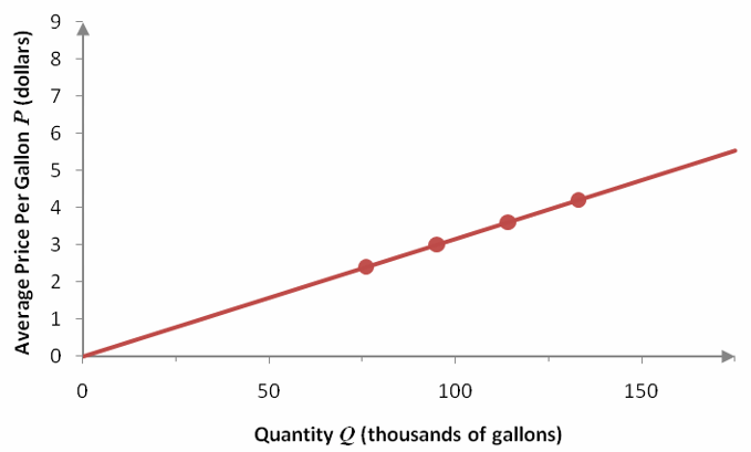
Figure 12 – Data from the supply schedule and the corresponding supply curve.
Keep in mind that while this is a “typical” supply schedule, supply functions may have many different shapes. A supply function may be curved concave down or up. It may even change its concavity.
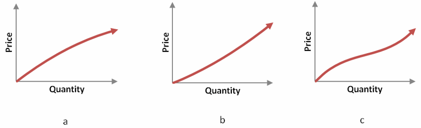
Figure 13 – Three examples of supply functions. In a, the supply curve is concave down. In b, the supply curve is concave up. In c, the supply curve changes from concave down to concave up.
A linear function often models the data adequately and simplifies later calculations. A linear supply function has the form
S(Q) = mQ + b
where m is the slope of the line and b is the vertical intercept.
Example 7 Find the Supply Function for Milk
Find the linear supply function S(Q), where Q is the quantity of milk supplied, passing through the ordered pairs in Table 7.
Solution Since the function will be a function of Q, interchange the columns of the table. This change is necessary since the independent variable is typically listed in the first column.
Let’s check the slope between adjacent points.
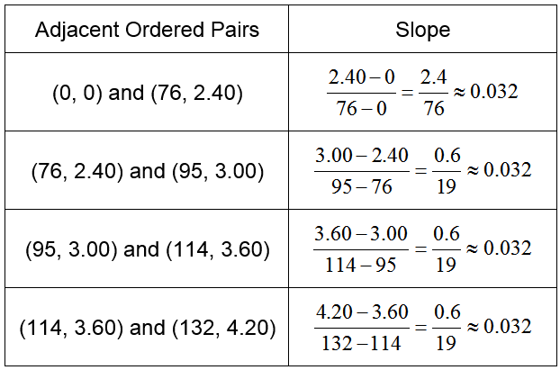
Table 8
The fractions 2.4/76 and 0.6/19 simplify to 3/95. Since all of the slopes are the same at about 0.032, we know the points lie along a straight line.
Unlike the demand function, we know that the vertical intercept is (0, 0) so the equation of the line is
![]()
Notice that the fraction has been used for the slope. If the rounded decimal had been used instead of the exact fraction, the line would go very close to the data in the supply schedule, but not through exactly. Decimals are acceptable when they are exact decimals and not rounded or where approximations are acceptable.
Example 8 Find the Surplus at a Fixed Price
At a price of $3.36 per gallon, dairies will be willing to supply more milk than consumers are willing to buy. Find the surplus amount of milk at this higher price.
Solution To find the amount of the surplus, we must find the difference between the quantity supplied and the quantity demanded. These quantities are found by setting the outputs of the supply and demand functions equal to $3.36.
To find the quantity supplied, set S(Q) equal to 3.36 and solve for the quantity Q :
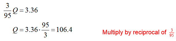
At a price of $3.36 per gallon, the dairies would be willing to supply 106.4 thousand gallons or 106,400 gallons of milk per week.
To find the quantity demanded by consumers, set D(Q) equal to 3.36 and solve for Q:
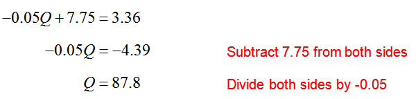
The demand at a price level of $3.36 per gallon is 87,800 gallons of milk per week.
The surplus of milk is the difference between the two quantities or
Surplus = 106,400 – 87,800 = 18,600 gallons per week