How good is the linear model?
The linear model is not complete without an indication of how good the fit is to the data. We can examine the scatter plot with the model and data and get a qualitative idea of the fit, but this can be deceiving.
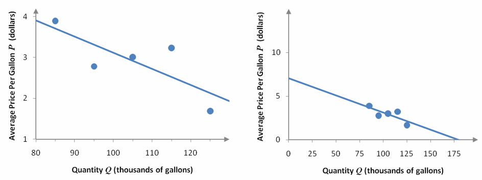
Figure 8 – Two scatter plots of the data in Table 1. The model of each scatter plot is P = -0.0395Q + 7.0675, but the horizontal and vertical scales are different.
Which linear model in Figure 8 appears to be a better fit? On the surface, you would probably say that the model on the right is a better fit. But in fact, both scatter plots depicts the exact same model with different scales. The vertical scale for the scatter plot on the right is larger and makes any gaps between the model and the data seem small. This makes the points appear to be closer to the line. In fact, the vertical distance between each data point and the line are exactly the same and there is no difference in the fit.
To remedy this and other difficulties in determining goodness of fit, two indicators are used. The correlation coefficient and coefficient of determination are commonly used to compare the fit of regression models.
The correlation coefficient r is a number from -1 to 1 that indicates how well the linear model fits a set of data. If |r| is closer to 1, the relationship between the data is more linear. If |r| is closer to 0, the data are not linearly related.
A positive correlation coefficient indicates that the data is positively correlated. For linear models with a positive correlation coefficient, the slope of the model will be positive. A negative correlation coefficient indicates that the data is negatively correlated. For linear models with a negative correlation coefficient, the slope of the model will be negative.
Figure 9 – Three different sets of data and the corresponding linear models. The worst fit is in graph a with an absolute value of the correlation coefficient closest to 0. The best fit is graph c with an absolute value of the correlation coefficient closest to 1. Each model is decreasing so the correlation coefficient is negative.
As |r| gets closer to 1, the data points get closer to the linear model.
Another measure of fit is the coefficient of determination, r2. For a linear model, the coefficient of determination is the square of the correlation coefficient . Since is a number from -1 to 1, r2 is a number from 0 to 1. The closer the coefficient of determination is to 1, the more linearly related the data are. If the coefficient of determination is close to 0, the data are not linearly related.
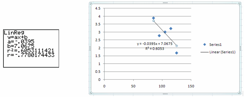
Figure 10 – A graphing calculator or Excel can be used to calculate the correlation coefficient or coefficient of determination. A graphing calculator (left) returns both values. Excel (right) can return the coefficient of determination (it is written as R2 instead of r2).
Another measure of how close the data lie with respect to the linear model is the percent error. The percent error at any value of the independent variable is found by dividing the error, , by the data value P. We can find the percent error by calculating
at each data value where P is the price data and is the model’s estimate of the price. At Q = 115, the percent error is
or approximately 21.8%. This means that as a proportion of the price, the price at Q = 115 is 21.8% above the model’s estimate of the price.
Example 3 Find the Largest Percent Error
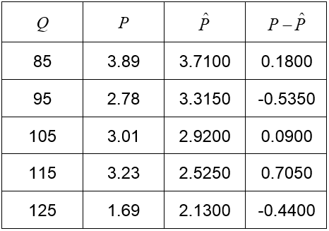
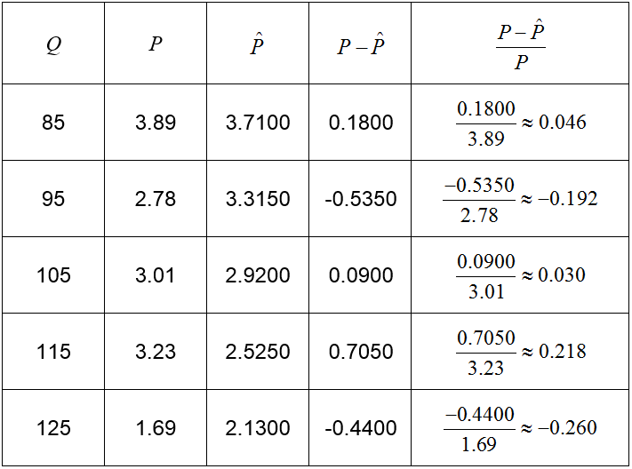
For the model P = -0.0395Q + 7.0675 and the data in Table 3,
Find the quantity that yields the largest percent error.
Solution Add a column to the table and calculate the percent error at each quantity.
The largest percent error is 26% and occurs at Q = 125. This price is 26% below the linear model.
