What is a derivative?
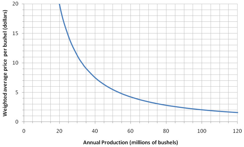
The derivative of a function at a point is closely related to the average rate of change of a function. To understand this relationship geometrically, let’s look at average rate of change of a function in the context of the slope of a secant line. We’ll use the graph below to illustrate this relationship. This graph shows the weighted average price per bushel for oats in dollars as a function of the annual production of oats in the United States in millions of bushels.
Figure 1 – The demand function describing the relationship between the annual production of oats and the weighted average price of oats.
This function decreases since the price drops as the annual production increases. This behavior is typical of demand functions.
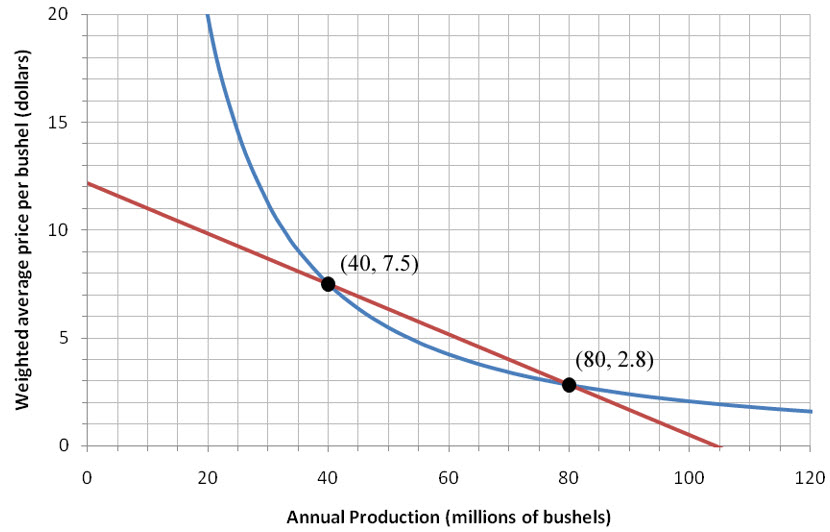
The average rate of change of the price per bushel with respect to annual production is found by calculating the change in the weighted average price per bushel, ΔP, and dividing that value by the change in the annual production, ΔQ. The average rate of change of weighted average price from an annual production level of 40 million bushels to 80 million bushels is
Since the numerator has units of dollars and the denominator has units of millions of bushels, the units on the average rate of change are of dollars per million bushels. The average rate of change is the same as the slope of the secant line, so the slope of the secant line in Figure 1 is -0.1175.
Figure 2 – The demand function for oat production (blue) with a secant line (red) passing through the production levels of 40 and 80 million bushels.
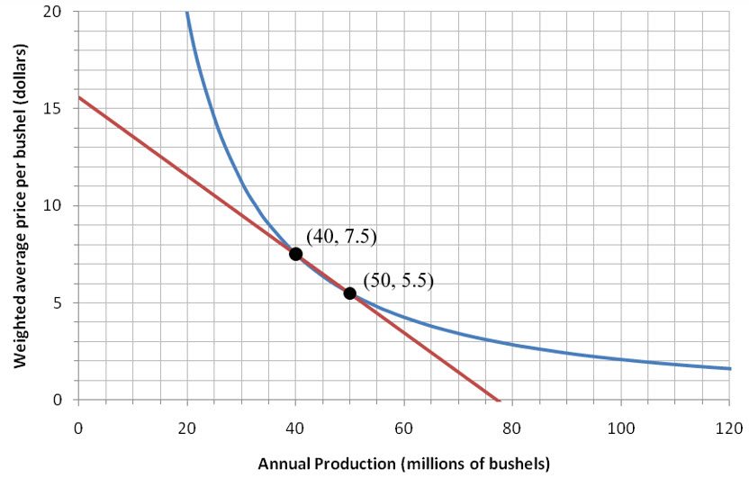
We are interested in approximating the instantaneous rate of change of the price with respect to the annual production at an annual production level of 40 million bushels. To do this, we need to find the average rate of change of the price over smaller and smaller changes in production near an annual production level of 40 million bushels. If we calculate the average rate of change between 40 and 50 million bushels instead of 40 and 80 million bushels, we obtain
This average rate of change is identical to the slope of the secant line passing through (40, 7.5) and (50, 5.5) pictured in Figure 2.
Figure 3 – The demand function for oat production (blue) with a secant line (red) passing through the production levels of 40 and 50 million bushels.
We can continue to find the average rate of change in price with respect to the change in annual production for smaller and smaller intervals. The average rate of change of price with respect to a change in annual production from 40 million bushels to 45 million bushels is
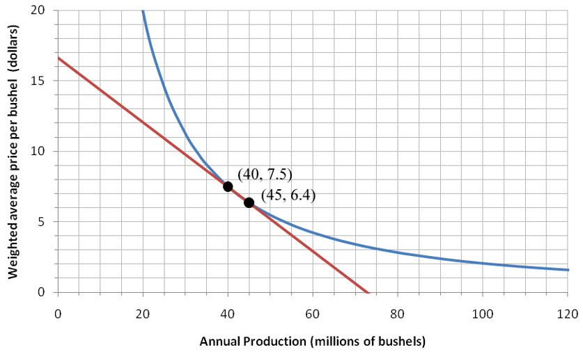
The slope of the secant line passing through (40, 7.5) and (45, 6.4) is also -0.22. This secant line is graphed with the demand function in Figure 3.
Figure 4 – The demand function for oat production (blue) with a secant line (red) passing through the production levels of 40 and 45 million bushels.
As we calculated the average rate of change of prices with respect to annual production for smaller and smaller changes in annual production, the values became more negative. If we continue to calculate the average rate of change for even smaller changes in production, will the value continue to become more negative or will the value get closer and closer to some negative number?
To answer this question, let’s take the average rate we have calculated so far, add a few more, and look for any patterns.
The average rate of change appears to be getting closer to a number as the change in production becomes smaller. However, it is difficult to see what that number is by simply calculating slopes of secant lines from points read off the graph.
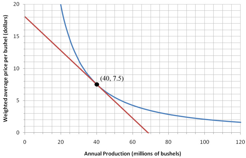
As the points on the secant line get closer and closer together, they become indistinguishable from each other on the graph. The secant line now appears to graze the graph at the point (40, 7.5). This line is called the tangent line to the function at that point.
Figure 5 – The demand function for oat production (blue) with the tangent line (red) at a production level of 40 million bushels.
As the change in production level was decreased, the secant line looked more and more like the tangent line. At the same time, the average rate of change of price with respect to a change in annual production became a better and better approximation of the instantaneous rate of change of price with respect to a change in annual production. Recalling that the instantaneous rate of change at a point is also called the derivative at that point, we define the following.
The tangent line to a graph f at a point (a, f (a)) is a line with slope f ′ (a) that passes through the point (a, f (a)).
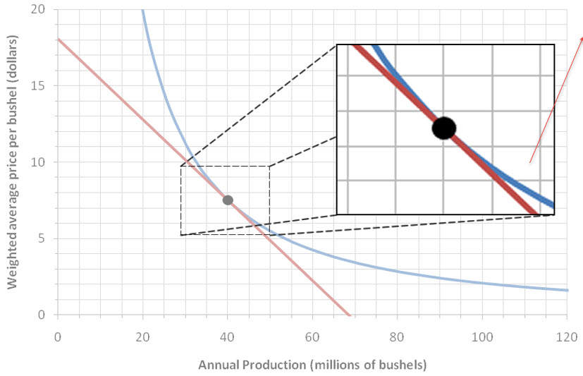
If we zoom in on the point (40, 7.5), we can see that the demand function and the tangent line are almost the same. Since the tangent line looks very much like the function near the point, we often say that the derivative f ′ (a) is the slope of the curve at the point (a, f (a)).
Figure 6 – The demand function for oat production (blue) and the tangent line (red) are almost indistinguishable when we zoom in on the point (40, 7.5).
Example 1 Estimate the Derivative at a Point
The function P = f (Q), pictured below, describes the weighted average price of oats per bushel in dollars as a function of the annual oat production in millions of bushels.
Figure 7 – The weighted price of a bushel of oats as a function of the annual production.
Use a tangent line to estimate the value of the derivative at Q = 40.
Solution The tangent line at Q = 40 is a line that looks most like the function P = f (Q) at that point.
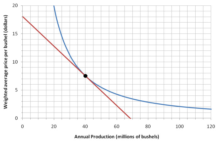
Figure 8 – The demand function for oats (blue) with a tangent line at Q = 40.
The slope of the tangent line at Q = 40 is equal to f ′ (40). If we estimate the location of two points on this line, we can calculate the slope between these points.
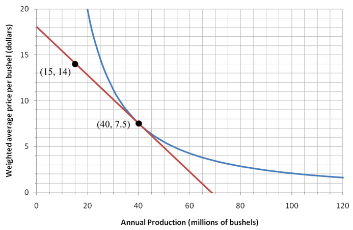
Figure 9 – The tangent line to the demand function with two points estimated.
We locate the points (15, 14) and (40, 7.5) from the graph. The slope msecant between the points is
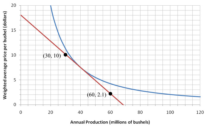
Any two points on the tangent line at Q = 40 may be used to estimate the slope of the tangent line. Different points may lead to slightly different estimates for the slope.
For instance, if we approximate the points (30, 10) and (60, 2.1) on the tangent line, we calculate the slope to be
Figure 10 – The tangent line with two different points estimated on the line.
Because we are locating the ordered pairs using the grid on the graph, the values are only guesses at the exact positions. We shouldn’t expect the estimates to be exactly the same. But in this case, careful estimation of the point’s locations leads to similar estimates.
