
What is a derivative function?
Let’s examine the tangent line on the function pictured in Figure 1.
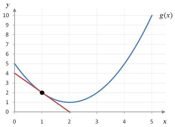
Figure 1 – A quadratic function g(x) (blue) with a tangent line (red) at x = 1.
We can approximate the value of the derivative at x = 1 or g′(1) by calculating the slope of the tangent line at x = 1. Any two points on the tangent line can be used to make an estimate of the slope.
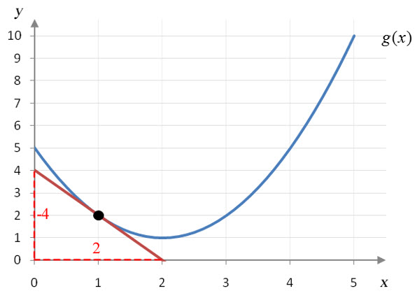
Figure 2 – The points (0, 4) and (2, 0) can be used to estimate the slope of the tangent line at x = 1.
From Figure 2, we see that the slope of the tangent line or g′(1) is approximately -4/2 or -2. Any other two points on the line could be used to calculate this slope. For instance, the points (1, 2) and (2, 0) are on the tangent line. The slope between these points is
$$ g’\left( 1 \right) \approx \frac{{2 – 0}}{{1 – 2}} = – 2 $$
Different points don’t always lead to exactly the same slope, but they should be close. If we look at the tangent line for g(x) at x = 2, we see that it is horizontal and passes through the point (2, 1).
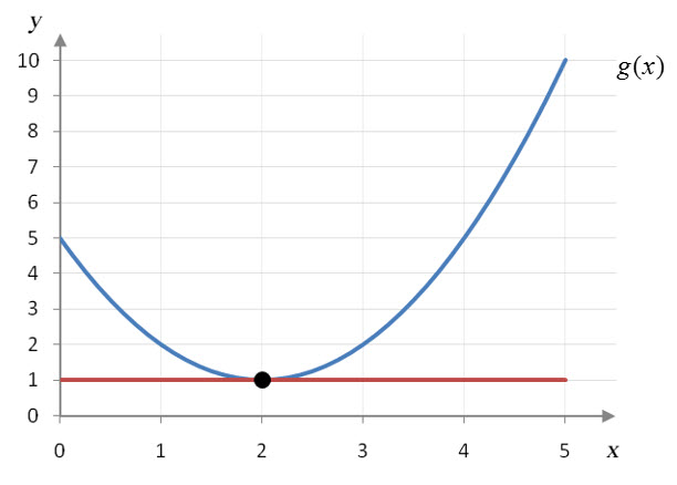
Figure 3 – The tangent line to g(x) at x = 2 is a horizontal tangent line.
Since the tangent line is horizontal, its slope is zero. This tells us that g′(2) = 0.
Let’s estimate the slope of one more tangent line at x = 4.
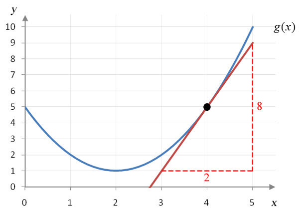
Figure 4 – The tangent line to g(x) at x = 4 passes through the points (3,1) and (5,9).
The slope is calculated as
$$g’\left( 4 \right) \approx \frac{{9 – 1}}{{5 – 3}} = \frac{8}{2} = 4$$
With these three tangent lines, we can organize the slopes in a table.
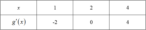
If we graph these values with the x values as the independent variable and the slopes as the dependent variable, we see a pattern emerge.
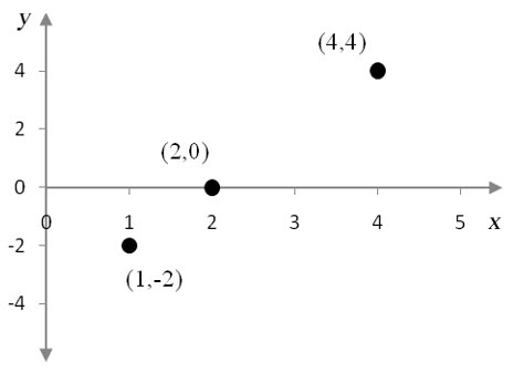
Figure 5 – In this graph, the slopes of the quadratic function are graphed at corresponding x values.
The slopes appear to lie along a straight line. If we draw this line through the points we can use it to find the slope of the tangent line at other x values.
Figure 6 – Each of the slopes of the quadratic function lie along a straight line.
For instance, at x = 3 the line passes though y = 2 . This means the slope of the tangent line at x = 3 on the quadratic function is 2. The function corresponding to this line is called the derivative of the quadratic function g(x) and is denoted by g′(x).
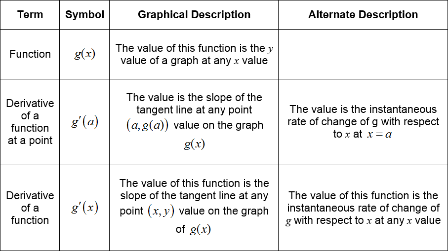
All of these concepts can be a bit confusing. So let’s recap these different ideas using a function g(x). Keep in mind that we could use any name in place of g and any variable in place of x.
Example 1 Find the Derivative Function
The graph of the function f (x) is shown below.
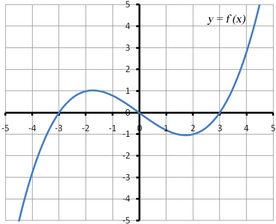
Find the graph of the derivative function f ′(x) using the tangent lines to the function f (x).
Solution To find the derivative of the function, we’ll draw tangent lines along the function, record the slopes in a table and graph the corresponding ordered pairs.
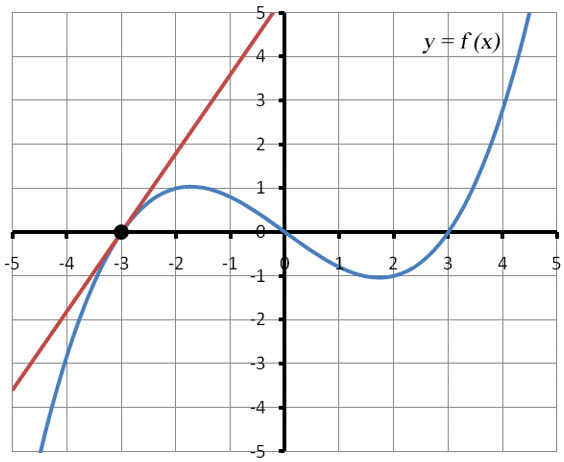
Using the grid on the graph, we see that the tangent line passes through (-3, 0) and (-2, 1.8). The slope of the tangent line is approximately
$$f'( – 3) = \frac{{1.8 – 0}}{{ – 2 – ( – 3)}} = 1.8$$
We’ll continue to fill out the table of tangent line slopes:
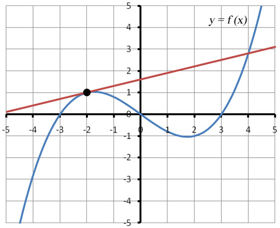
Our ability to calculate the slope is constrained by our ability to locate points on the tangent line. For this tangent line, the points (-2, 1) and (1, 1.9) are on the line. The slope of the tangent line is approximately
$$f'( – 2) = \frac{{1.9 – 1}}{{1 – ( – 2)}} = 0.3$$
At the next row in the table, we find the slope of the tangent line at x = -1:
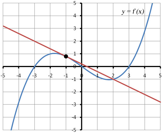
Any two points on the tangent line can be used to find the slope. For this tangent line, the points (-3, 2) and (2, -1) are on the line. The slope of the tangent line is approximately
$$f'( – 1) = \frac{{ – 1 – 2}}{{2 – ( – 3)}} = – 0.6$$
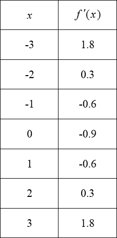
If we continue to find the slopes of tangent lines at each of the x values in the table, we can graph the ordered pairs in the form (x, f ′(x)). This means that we graph the x values horizontally and the f ′(x) values vertically.
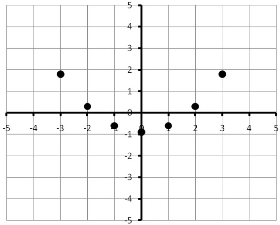
These ordered pairs lie on the derivative function f ′(x).
If we were to graph more points on the derivative function, we would see a graph like the one below.
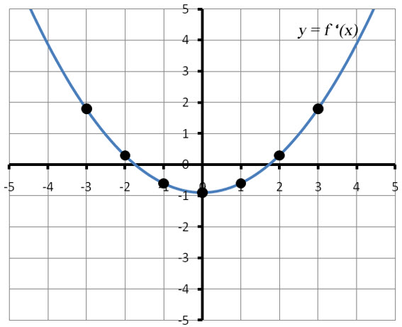
Usually it is not necessary to graph a large number of points to graph the derivative function. Typically a few points on the graph are enough to display the overall pattern. Then the rest of the graph can be sketched to approximate the pattern.