
How do we make decisions about inventory?
Most businesses keep a stock of goods on hand, called inventory, which they intend to sell or use to produce other goods. Companies with a predictable demand for a good throughout the year are able to meet the demand by having an adequate supply of the good. A large inventory costs money in storage cost and carrying low inventory subjects a business to undesirable shortages called stockouts. A company’s inventory level seeks to balance the storage cost with costs due to shortages.
 A light emitting diode (LED) is a light source that is used in many lighting applications. In particular, LEDs are used to produce very bright flashlights used by law enforcement, fire rescue squads and sports enthusiasts. Suppose a manufacturer of LED flashlights needs 100,000 LED bulbs annually for their flashlights. The company may manufacture all of the LED bulbs at one time or in smaller batches throughout the year to meet its annual demand. If the manufacturer makes all of the bulbs at one time they will have a supply to make flashlights throughout the year, but will need to store bulbs for use later in the year. On the other hand, if they make bulbs at different times throughout the year, the factory will need to be retooled to make each batch.
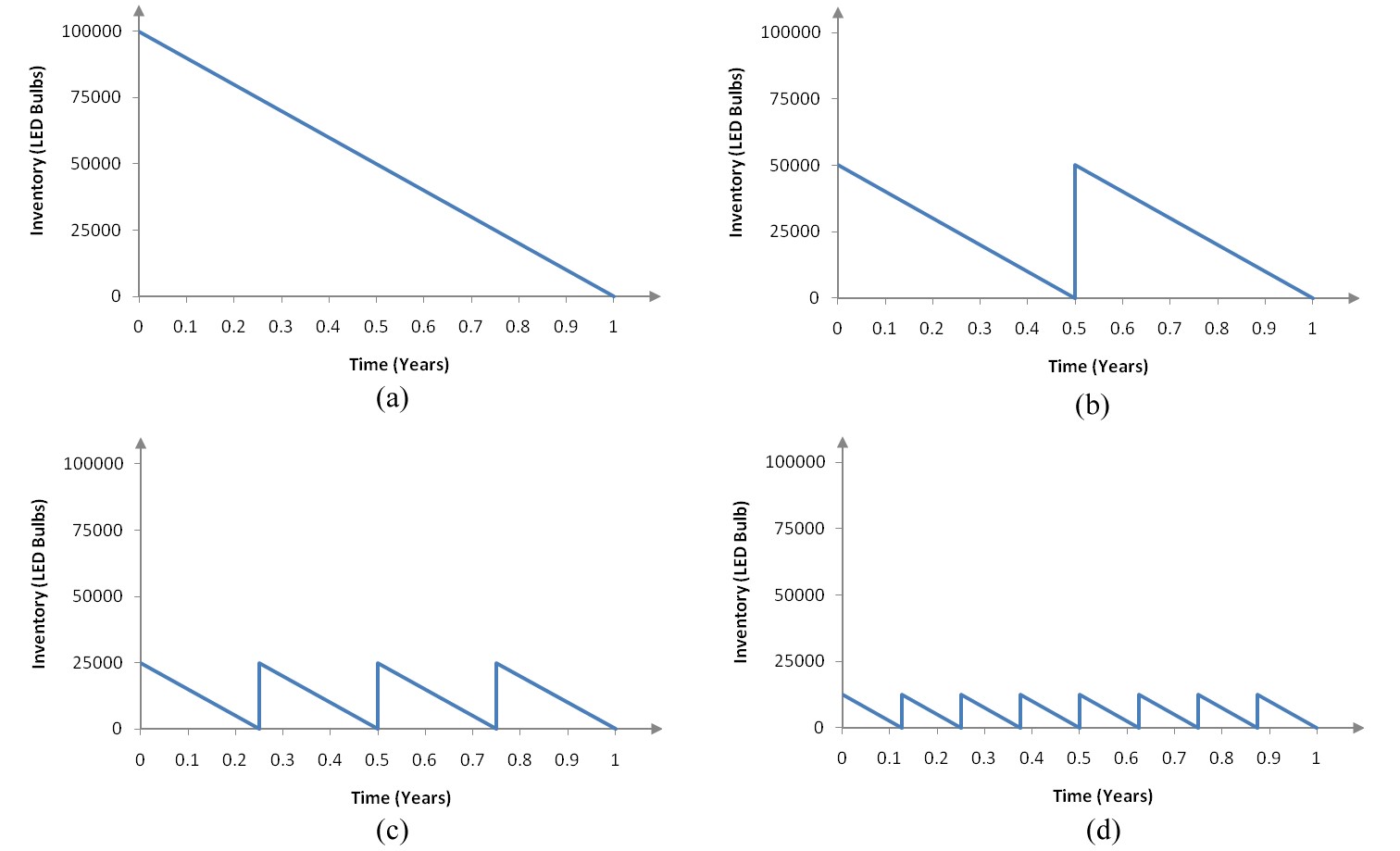
Figure 1 – Inventory levels at the manufacturer over a one year period. In (a), all bulbs are made at the beginning of the year and used at a constant rate throughout the year. In (b), two batches of 50,000 are made. In (c), 4 batches of 25,000 are made. In (d), 8 batches of 12,500 are made. In each case, when the inventory reaches 0, the next batch is manufactured instantaneously.
Since the manufacturer does not need to make LED bulbs continuously throughout the year, they will use the manufacturing capacity for other purposes during the rest of the year. When they do manufacture the bulbs, the factory will need to be set up for this purpose. For this manufacturer, it costs 5000 dollars to set up the factory to manufacture LED bulbs. This amount covers all costs involved in setting up the factory such as retooling costs, diminished capacity while the production line is retooled, and labor costs. Each time the company manufactures a batch of bulbs, they incur this cost. Obviously, the more times the plant retools, the higher the total cost is.
The company pays a holding cost to store any LED bulbs not used. The holding cost includes the taxes, insurance, and storage costs that change as the number of units stored changes. If they manufacture all of the bulbs at one time, they will have to store more bulbs throughout the year. For this manufacturing plant, it costs $1 to hold a bulb for one year.
We’ll assume that the company’s production cost does not change throughout the year. In other words, whether they manufacture the bulbs all at once or in several batches throughout the year, it will cost them the same amount per unit to manufacture the bulbs. For this plant, it costs 25 dollars to manufacture an LED bulb.
The total cost for the manufacturer is the sum of the set up, holding and production costs. For other manufacturers, other costs may be included in this sum. However, we’ll assume that the total cost for this plant is restricted to these three costs. If they produce more LED bulbs in each batch, the set up costs will be lower but they will pay a higher holding cost. On the other hand, if they produce fewer bulbs in each batch they will lower the holding cost. This decrease in holding cost is accompanied by an increase in the set up cost since more batches will be needed to meet the annual demand. The manufacturer faces a simple question: how many units should they manufacture in each batch so that their total cost is minimized? The batch size that results in the lowest total cost is called the economic lot size.
Example 3 Find the Economic Lot Size
A manufacturing plant needs to make 100,000 LED bulbs annually. Each bulb costs 25 dollars to make and it costs 5000 dollars to set up the factory to produce the bulbs. It costs the plant 1 dollars to store a bulb for 1 year. How many bulbs should the plant produce in each batch to minimize their total costs?
Solution To find the economic lot size, we need to analyze the costs for the plant and model these costs.
What kind of costs will be incurred? Three different types of costs are described in this example. A set up cost of 5000 dollars is incurred to set up the factory. A production cost of 25 dollars per bulb is incurred for labor, materials, and transportation. Since the demand for bulbs occurs throughout the year, we’ll need to store some of them in a warehouse at a holding cost of 1 dollar per bulb for a year.
Let’s try to solve this naively and simply produce all 100,000 bulbs in one batch. If the demand throughout the year is uniform, we can expect to have an average inventory of
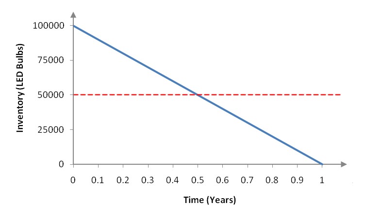
Figure 2 – If all of the LED bulbs are produced in one batch, the average inventory is 50,000 bulbs.
It will cost 1 dollar to store each of these bulbs for holding costs of 50,000 × 1 dollar or 50,000 dollars. If all of the bulb are produced in one batch, the production line will need to be set up once for a cost of 5000 dollars.To produce 100,000 bulbs at a cost of 25 dollars per bulb will cost 100,000 × 25 dollars or 2,500,000 dollars. The total cost to produce one batch of 100,000 bulbs is the sum of these costs,
The largest cost in this sum is the production cost. If the cost to make a bulb is fixed and we don’t change the number of bulbs produced each year, changing the batch size won’t affect this term.
We can lower the holding cost by producing fewer bulbs in each batch. But this increases the set up cost since the production line will need to be set up more often.
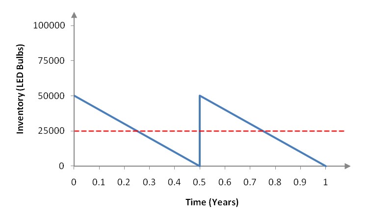
Figure 3 -If the LED bulbs are produced in two batches, the average inventory is reduced to 25,000 bulbs.
If the batch size is reduced to 50,000, the average inventory is reduced to
for storage costs of 25,000 × 1 dollar or 25,000 dollars. The production line will need to be set up twice at a cost of 2 × 5000 dollars or 10,000 dollars.
We will still produce 100,000 bulbs at a cost of 25 dollars per bulb. This will cost 100,000 × 25 dollars or 2,500,000 dollars. The total cost is now
In this case, the holding cost dropped by 25,000 dollars, but the set up cost increased by 500 dollars. This results in a lower total cost.
Continuing with this strategy, we can fill out the following table:
As the lot size decreases, the set up cost increases and the holding cost decreases. Initially, the holding cost is much higher. But for smaller batch sizes, the set up cost is much higher. Somewhere in the middle is a batch size whose total cost is as small as possible.
To find the batch size Q that minimizes the total cost, we need to find a function that models the total cost as a function of Q. Examine the patterns in the table. Each set up cost in the second column is a product of 5000 dollars and the number of batches that will be produced. We get the number of batches by dividing 100,000 by the batch size, ![]() . This means a batch size of Q will have a set up cost of
. This means a batch size of Q will have a set up cost of
In every row of the second column, the production cost is the same. So changing the size of the batch has no effect on the production cost.
The holding cost is the product of the average inventory and the unit holding cost. If the batch size is Q, the holding cost is
![]()
Let’s add these expressions to the table.
Notice that the expression in the last row for the total cost preserves the pattern for all values of Q above it.
The total cost as a function of the batch size Q is
Before we take the derivative to find the critical points, let’s simplify this function,
Using the Power Rule, the derivative is computed as
Notice that the production cost drops out of the critical point calculation meaning the production cost has nothing to do with the economic lot size. This function is undefined at Q = 0. But a batch size of 0 is not a reasonable answer since a total of 100,000 bulbs must be made.
More critical points can be found by setting the derivative equal to 0 and solving for Q:
Only the quantity 31,623 bulbs makes sense. But is this critical point a relative minimum or a relative maximum?
To check, we’ll substitute the critical point into the second derivative and determine the concavity at the critical point. Starting from the first derivative, ![]() , the second derivative is
, the second derivative is
At the critical point,
The second derivative is positive since the numerator and denominator are both positive. A function that has a positive second derivative at a critical point is concave up. This tells us that Q = 31,623 is a relative minimum. The total cost at that point is
A lot size of approximately 31,623 bulbs leads to the lowest total cost possible of 2,531,622.78 dollars.
Some companies purchase their inventory from manufacturers. Instead of deciding how many units to manufacture in each batch, they must decide how many units they should order and when they should order the units. For a business like this, the set up cost is replaced by the ordering cost.
The ordering cost includes all costs associated with ordering inventory such as developing and processing the order, inspecting incoming orders, and paying the bill for the order. Larger companies may also have purchasing departments. The ordering cost also includes the cost of the personnel and supplies for the purchasing department.
Ordering more often lowers holding cost since it results in lower inventory levels. This also raises ordering cost since more orders must be placed. The total cost is minimized at an order size that balances the ordering cost and the holding cost. This order size is called the economic order quantity.
Example 4 Find the Economic Order Quantity
 The annual demand for a particular wine at a wine shop is 900 bottles of wine. It costs 1 dollar to store one bottle of wine for one year. It costs 5 dollars to place an order for a bottle of wine. A bottle of wine costs an average of 15 dollars. How many bottles of wine should be ordered in each order to satisfy demand and to minimize cost?
Solution Upon examining this problem, it might appear that the wine shop should simply order 900 bottles of the wine once a year. While this is a possible solution and lowers the ordering cost, it would incur a large holding cost. The wine shop could also place 18 orders of 50 bottles each. This would lower the holding cost, but increase the ordering cost. Another possibility would be to order each bottle individually. This would lower the holding cost even more, but increase the ordering cost. The appropriate order size will balance the holding cost and the ordering cost so that the total cost is as small as possible.
To solve this problem, we need to find a total cost function. Once we have this cost function, we’ll take the derivative of the function to find the critical points and locate the relative minimum. For this problem, we need to vary the order size to see the effect on the costs. For this reason, the variable in this problem will be the order size Q. Let’s calculate the costs for several different values of Q to see the relationship between the order size and the total cost.
Suppose we make a single order of 900 bottles of wine. Since we are making a single order, the ordering costs will be 5 dollars. However, it will take the entire year for all of these bottles to be sold. The average amount on hand will be
Thus the storage costs will be 450 bottles ×1 dollar per bottle to store. Each bottle of wine costs an average of 15 dollars, so 900 bottles will cost 900(15 dollars) or 13,500 dollars.
The total cost is
![]()
If we make two orders of 450 bottles each, the reordering cost will be 2×5 dollars and the storage costs will be 225 bottles ×1 dollar per bottle. Assuming the cost of the wine does not change throughout the year, the wine will still cost 13,500 dollars. For this order size, the total ordering cost is
![]()
Using this strategy, we can fill out the table below:

Look at each line of this table. As the order size decreases, the reordering costs increase and the storage costs decrease. The sum of all costs starts at 13955 dollars and decreases initially as the storage costs drop. However the reordering costs begin to build up eventually causing the total ordering cost to increase to 4500.50 dollars for an order size of 1 bottle.
Based on the table, we can guess that an order around 50 bottles might lead to the lowest total ordering cost. To make this more exact, we need to find the total cost as a function of the order quantity Q. The ordering cost come from the number of orders times the cost per order. We can find the number of orders by dividing 900 by the order size or ![]() . The ordering cost is
. The ordering cost is
The holding cost are simply the average inventory times the cost per bottle to store or
![]()
The total cost function is the sum of these costs and the cost of the wine,
Let’s add these quantities to our table to see how they match up with the numbers we found before:
Each ordering cost in the second column consists of the 5 dollars cost to order times a value. This value is the number of orders you will need to make during the year. Each holding cost in the third column consists of the 1 dollar cost to store one bottle for one year, times the average inventory. The expression we have written for the total costs preserves these patterns.
Before we find the critical points of TC(Q), let’s simplify the function to make the derivative easier to find. Carry out the multiplication in the first term and use negative exponents in the first term to give
![]()
The derivative of this function is
To find the critical points, we need to find where the derivative is undefined or equal to 0. This function is undefined at Q = 0, but an order size of 0 is not a reasonable order since we need 900 bottles annually. Setting the derivative equal to 0 and solving for Q yields
This is approximately ±94.87. Clearly, a negative order size makes no sense. The only reasonable critical point for this function is . To insure that this is a relative minimum and not a relative maximum, we’ll apply the second derivative test. The second derivative is
At the critical point, the second derivative is
![]()
so the original function TC(Q) is concave up. The critical point at Q ≈ 94.87 is a relative minimum.
Should the wine shop order 94.87 bottles of wine? Bottles of wine are sold in integer amounts so we have two options: order 94 bottles (and not meet the demand) or order 95 bottles (and have a few bottles extra at the end of the year). You might choose to order 95 per order to simply insure that you satisfy all customers, but which option is cheapest?
In deciding which option is better, you’ll need to balance what is the biggest benefit and what are the costs of the decision. In this case, an order size of 95 is slightly cheaper than an order size of 94 and ensures that all customers are satisfied.