Where do systems of equations come from?
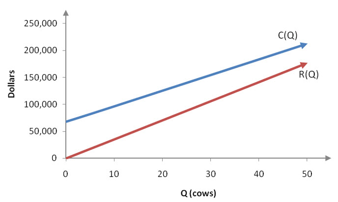
In Examples 4 and 5 of section 1.2, we found the total cost C(Q) and the total revenue R(Q) for a dairy as a function of the number of cows, Q. The total cost function, C(Q) = 2890.8Q + 68688, and the revenue function, R(Q) = 3547Q, are graphed in Figure 5.
Figure 5 – Revenue and cost functions for the dairy.
As the number of cows at the dairy is increased, the cost to maintain the dairy and the revenue from dairy products both increase. In the window shown in Figure 5, the two graphs do not intersect. But the revenue function has a slope of 3547 and the cost function has a slope of 2890.8. Since the revenue function is steeper than the cost function they will eventually intersect.
We can form a system of equations whose solution corresponds to the point of intersection by replacing the function notation with a variable. Let Y represent the amount of money in dollars and use Y to replace both R(Q) and C(Q). This is reasonable since both functions output amounts of money in dollars. The system
allows us to see the relationship between the revenue and cost for a business. By graphing this system, we can interpret what the point of intersection means in the context of the dairy and other types of businesses.
Example 6 Find the Point of Intersection for the Dairy
Graph the system of equations
to find the solution to the system.
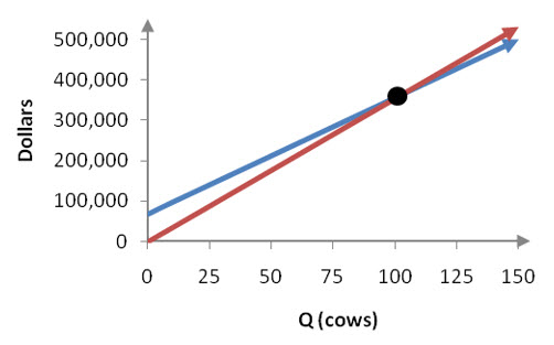
Solution Each equation in the system is solved for the dependent variable Y and can be graphed directly.
Figure 6 – The system of equations representing the cost (blue) and revenue (red) of a dairy.
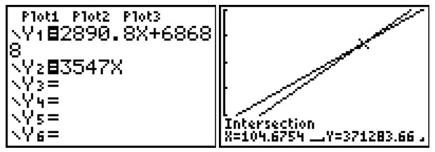
To find an estimate of the location of the point of intersection, we can use a graphing calculator or other type of technology.
Figure 7- Screenshot on a graphing calculator of the system of equations in Example 6.
The point of intersection is at Q ≈ 104.6754 and Y ≈ 371283.66. This tells us that at approximately 104.6754 dairy cows, the total cost of maintaining the herd is about $371,283.66 and the revenue generated by the herd is about $371,283.66. At this point, the total cost and revenue are exactly the same.
A break-even quantity of approximately 104.6754 dairy cows leads to an interesting point. Is it possible to have 0.6754 of a dairy cow? The quantity of cows Q must take on non-negative integer values. The dairy owner will have either 104 cows or 105 cows. Let’s examine the costs and revenue at each of these herd sizes.
At a herd size of 104,
the costs are slightly higher than the revenue by about 369,331,20 – 368,888 or 443.2 dollars. This indicates that the dairy would be losing money. In terms of profit, the dairy has a negative profit since the costs are greater than the revenue.
At a herd size of 105,
the revenue is slightly higher than the cost by about 372,435 – 372,222 or 213 dollars. The dairy is making money since the profit is $213 at this herd size.
Neither herd size results in the revenue equal to the cost. For realistic herd sizes, the revenue and costs are not exactly equal. However, a herd size of 105 is closer to the point of intersection.
The point at which a business’s costs and revenue are equal is called the break-even point. As demonstrated in Example 6, this point can be found by solving a system of equations consisting of a revenue equation and a cost equation.
In specifying a break-even point, we may find that the point of intersection is at an unrealistic value due to the nature of the items being produced. A complete analysis should examine the break-even point as well as realistic values for the variable near the break-even point.
We can also examine where other graphs intersect to find business-related quantities. In Chapter 1, we introduced supply and demand functions. The supply function S(Q) represents the price at which suppliers would be willing to supply Q products. The demand function D(Q) represents the price at which consumers would be willing to buy Q products. In a market, the demand by consumers and the supply by manufacturers may or may not be in balance.
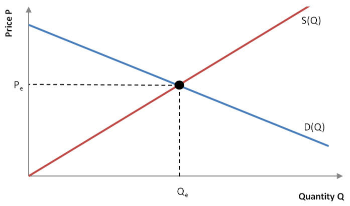
The quantity demanded by consumers may be in perfect balance with the quantity supplied by suppliers. At this price and quantity, called the equilibrium point, consumers demand the exact quantity that manufacturers are willing to supply. On a graph of the supply and demand functions, the equilibrium point is the point of intersection of the two graphs. This ordered pair is labeled (Qe, Pe), where the subscript refers to equilibrium.
Figure 8 – At the equilibrium point (Qe, Pe) the quantity demanded by consumers is matched by the quantity that manufacturers are willing to supply.
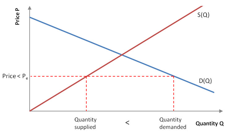
At prices lower than the equilibrium price, the quantity demanded by consumers is larger than the quantity supplied by manufacturers. In Figure 9, the red dashed horizontal line corresponds to a price that is lower than the equilibrium price. When the quantity demanded by consumers is larger than the amount supplied by manufacturers, there is a shortage of the product.
Figure 9 – If the price is below the equilibrium price, the quantity demanded by consumers is greater than the quantity that manufacturers are willing to supply. This results in a shortage of the item on the market.
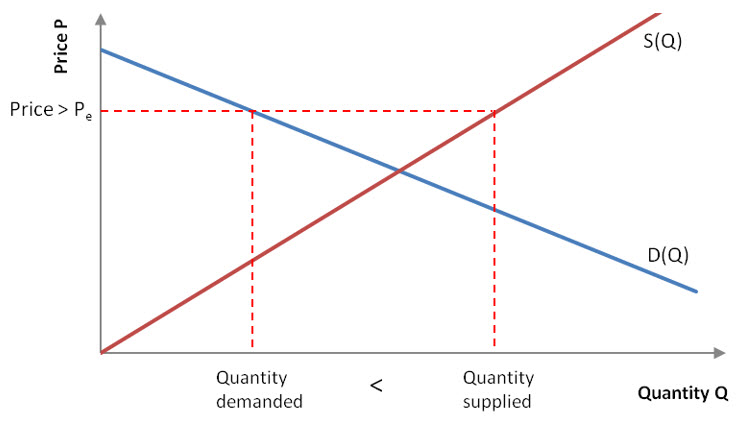
When the quantity that manufacturers are willing to supply is greater than the quantity the consumer is willing to buy, there is a surplus of the item on the market. A surplus occurs when the price of the product is greater than the equilibrium price.
Figure 10 – If the price is above the equilibrium price, the quantity supplied by firms is greater than the quantity that suppliers are willing to supply. This results in a surplus of the item on the market.
A surplus of an item will lead to lower prices since it costs businesses money to keep inventory on hand. The price will tend to lower until the price reaches the equilibrium price. At this point the quantity demanded by consumers and the quantity that manufacturers are willing to supply will be equal.
Example 7 Find the Milk Equilibrium Point
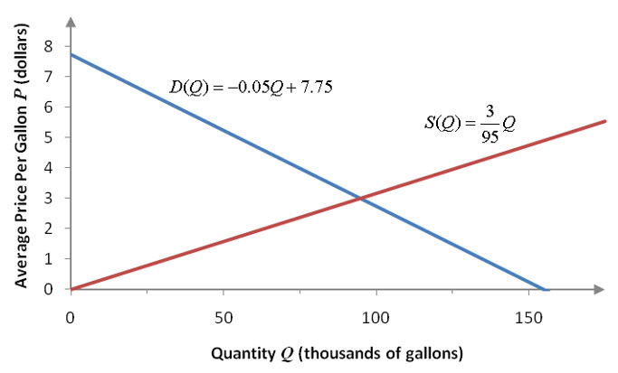
In earlier examples, we found the supply and demand functions pictured below for a small dairy.
Figure 11 – The demand function D(Q) and the supply function S(Q) for the dairy.
Find the equilibrium point for the dairy.
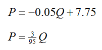
Solution The graph in Figure 11 shows an equilibrium point at roughly (100, 3). To find a better estimate of the equilibrium point, we need to utilize some sort of technology like a graphing calculator. Start by rewriting the functions D(Q) and S(Q) with a variable. Since the output from each of these functions is a price, we’ll use P. The system of equations is
The first equation relates the quantity of milk demanded by consumers to the price. As you would expect, higher quantities are demanded when the price is lower. The second equation relates the quantity of milk that dairy farms are willing to supply to the price. Higher quantities are supplied when the price is high.
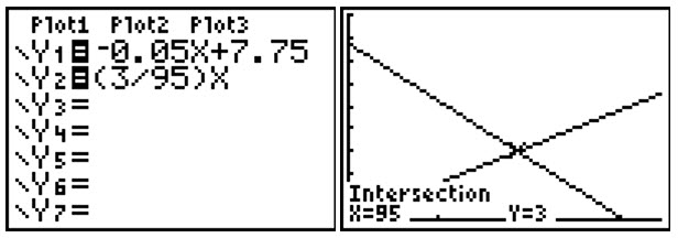
Figure 12 – A screen shot of the system of equations in Example 7. The equilibrium point is at (95, 3).
According to the estimate in Figure 7, at an average price per gallon of three dollars, 95,000 gallons of milk will be demanded by consumers and dairies will be willing to supply 95,000 gallons of milk. Since the demand and supply are in balance, this is the equilibrium point.
