How do you solve a linear programming application with a graph?
Now that we have established the strategy for solving linear programming problems graphically, let’s return to the two brewing examples.
Example 5 Solve the Linear Programming Application Graphically
The linear programming problem for a craft brewery is
where x1 is the number of barrels of pale ale and x2 is the number of barrels of porter produced. Solve this linear programming problem graphically to find the production level that maximizes the profit P.
Solution In earlier examples, we developed the system of inequalities and objective function for a craft brewery. By graphing many isoprofit levels we were able to find the optimal value for the profit function.
In this example we’ll use the simpler strategy we developed for maximizing the objective function. We’ll need to find the corner points of the feasible region and evaluate them in the objective function to find the maximum profit.
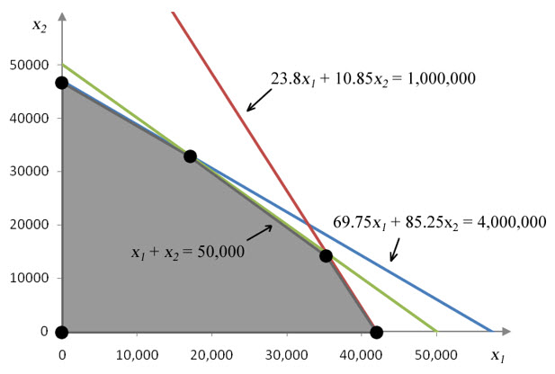
Figure 22 – The feasible region for the craft brewery.
The feasible region has five corner points that we must find. The easiest corner points to locate are the origin, the vertical intercept for 69.75x1 + 85.25x2 = 4,000,000 and the horizontal intercept for 23.8x1 + 10.85x2 = 1,000,000.
To find the vertical intercept for 69.75x1 + 85.25x2 = 4,000,000, set x1 = 0 and solve for x2:
The coordinates of this vertical intercept are approximately (x1, x2) = (0, 46920.8).
To find the horizontal intercept for 23.8x1 + 10.85x2 = 1,000,000, set x2 = 0 and solve for x1:
The coordinates of this horizontal intercept are approximately (x1, x2) = (42016.8, 0).
The other two corner points are points of intersection between the different borders. To find the corner point where the line x1 + x2 = 50,000 and the line 69.75x1 + 85,25x2 = 4,000,000 intersect, write this system of equations as the augmented matrix
We can use a graphing calculator or row operations to put this matrix into its reduced row echelon. The reduced row echelon form is
where the last column has been rounded to one decimal place. This places the corner point at approximately (16,935.5, 33,064.5).
The last corner point is located where the line x1 + x2 = 50,000 and the line 23.8x1 + 10.85x2 = 1,000,000 intersect. The augmented matrix for this system is
The reduced row echelon form for this matrix is
The third column has been rounded to one decimal place. This corresponds to the corner point (35,328.2, 14,671.8).
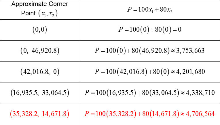
To find the production level that results in maximum profit, we need to substitute the corner points into the profit function.
The maximum profit is approximately $4,706,564 and is achieved when 35,328.2 barrels of pale ale and 14,671.8 barrels of porter are produced. The term “approximately” is used since the production levels have been rounded to the nearest tenth of a barrel.
Example 6 Solve the Linear Programming Application Graphically
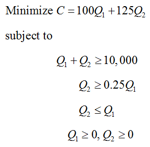
The linear programming problem for the contract breweries is
where Q1 is the number of barrels of American pale ale contracted at brewery 1 and Q2 is the number of barrels of American pale ale contracted at brewery 2. How many barrels should be contracted from each brewery to minimize the production cost C?
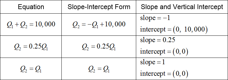
Solution To find the optimal production levels, we need to graph the feasible region and evaluate the corner points in the cost function. The borders of each inequality are given by the equations Q1 + Q2 = 10,000, Q2 = 0.25Q1, and Q2 = Q1. Each of these equations can be graphed by utilizing slope-intercept form, Q2 = m Q1 + b. In this form, Q1 is graphed horizontally, and Q2 is graphed vertically.
Utilizing this information, we can graph the borders.
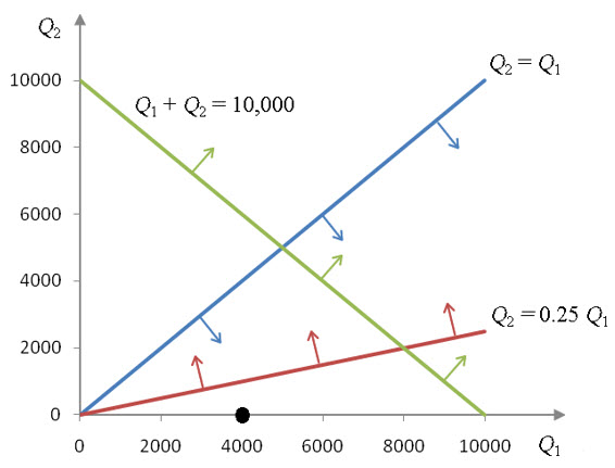
Figure 23 – The borders for the system of inequalities in Example 6.
The graph is shown in the first quadrant because of the non-negativity constraints Q1 ≥ 0 and Q2 ≥ 0.
To shade the solution for each inequality, we need to use a test point. Whenever possible we try to use (0, 0) for simplicity. However, this point is on two of the lines so we need to use another point. Any point can be used, and in this example we’ll use (4000, 0).
For the two inequalities that are false, we need to draw arrows on the lines pointing away from the test point. For the inequality that is true, we draw an arrow on the line pointing toward the test point. The arrows indicate the half planes that match the solution set of the individual inequalities.
Figure 24 – The individual solutions to the inequalities in Example 6.
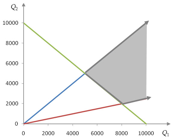
The solution sets for the individual inequalities in the system of inequalities overlap in the shaded region in Figure 25.
Figure 25 -The feasible region is unbounded since it cannot be enclosed in a circle. If a minimum cost exists, it will occur at one or both of the two corner points of the region.
This feasible region is unbounded since it cannot be enclosed in a circle. If a minimum cost exists, it will occur at one or both of the two corner points of the region.
To find the corner points, we need to solve the systems of equations formed by the borders that intersect at the corner point. For instance, if we solve
we can locate the point at which the green and blue lines cross. This is easy to do if we replace Q2 with Q1 and solve for Q1:
Since Q2 = Q1, the corner point is at (5000, 5000).
The other corner point corresponds to the solution of the system
Replace Q2 with 0.25Q1 and solve for Q1:
Since Q2 = 0.25Q1, we can calculate Q2 = 0.25 (8000) = 2000 to yield the corner point (8000, 2000).
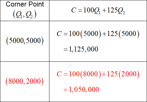
The optimal solution is found by evaluating the cost function at each of the corner points.
Figure 26 – The feasible region with the isocost line C = 1,050,000. Lower isocost lines are to the left of this line and outside of the feasible region.
The lowest cost is $1,050,000. It occurs when 8000 barrels from brewery 1 and 2000 barrels from brewery 2 are contracted.
