What is a frequency distribution?
A local bank is interested in tracking the time it takes a customer transaction to be completed. On Monday, they randomly select 20 customers and measure the amount of time it takes each customer to make a deposit. Each data value is rounded to the nearest minute.
Data like this is easy to record. As banks compete for customers, they strive to lower the amount of time it takes a customer to make a deposit.
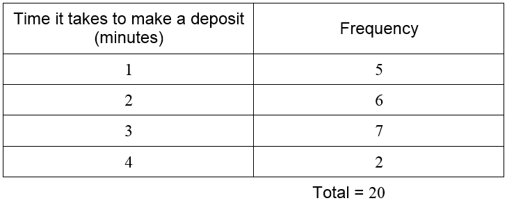
With only 20 numbers, it might be possible to examine the data and get some useful information about it. As more and more data is collected, the numbers become lost in the sheer amount of information. It is helpful to represent the data differently. A frequency distribution table allows us to see the different data values and how frequently they occur. The data in the table above are discrete data. This means they only take on a few values. In this case, the data only takes on the values 1, 2, 3, or 4. The frequency distribution table is constructed by counting the number of times each data value occurs. These frequencies are then listed with the corresponding data value in a table.
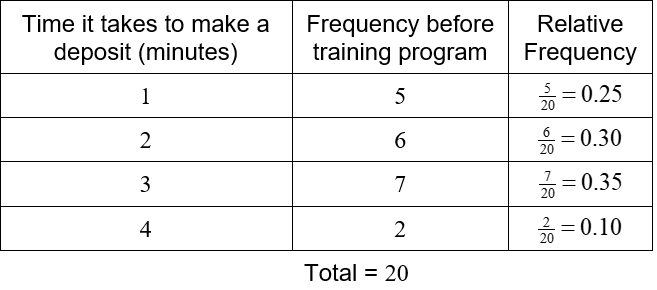
For instance, the data value 1 occurs 5 times in the table. The data value 2 occurs 6 times, 3 occurs 7 times, and 4 occurs 2 times. List these values in a table.
The total is often included to insure that all data values have been included in the count. Looking at the table, we see that the time of 3 minutes occurs most frequently. In fact, almost all deposits take 3 minutes of less.
Example 1 Find the Frequency Distribution Table
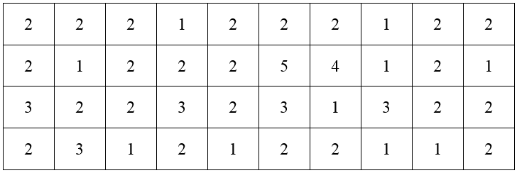
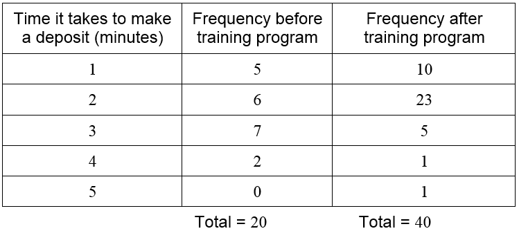
The bank develops a new training program to help make each teller more efficient. After all tellers have completed the training program, the bank measures the amount of time it takes 40 randomly selected customers to make a deposit. These times are recorded in the table below.
Construct a frequency distribution table for the data.
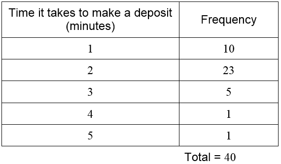
Solution The data in this table takes on the values 1, 2, 3, 4, and 5. We will need rows in the frequency distribution table for each value. Then count the number of times each value occurs and record the frequency.
The frequencies add to 40 so we have included all of the times in the table. Without this total, we would not know if we miscounted the data values.
Let’s compare the two frequency distribution tables we have created. Add another row to the first table for a deposit taking 5 minutes, but with a frequency of zero.
Since the totals for each table are different, it is harder to make a direct comparison of the tables. This is remedied by computing the relative frequency of each data. The relative frequency is computed by dividing each frequency by the corresponding total number of measurements.
To help us develop a framework for working with discrete data, suppose there are k different data values with k corresponding frequencies. In the case of the bank data, there are five different data values (1, 2, 3, 4, 5). We refer to any individual data value as xi where i can take on the values one through five. The frequencies are referenced as fi. For instance, we would call the first data value, 1, using x1. The corresponding frequency (either 5 or 10 depending on whether we are using the data before or after the training program) is f1. Using this notation, the sum of the frequencies for the first set of data is
For larger numbers of data values, writing a sum in terms of each individual frequency is cumbersome. Sigma notation is used to symbolize a sum. In this case, we would write
The Greek letter sigma (∑ ) is used to indicate a sum of some type. The individual terms of the sum are fi where i takes on the values 1 through 5. This notation may seem a little excessive for only five data values, but it comes in handy when you have 10 or more data values.
The relative frequency for the first data before the training program is
where n is the total number of measurements. Doing a similar calculation for the other frequencies before the training program gives us the table below.
The relative frequency is highest for a 3 minute deposit with 35% of the deposits taking this time. Ten percent of the deposits take 4 minutes. These percentages enable us to compare the data to other sets of data that may have a different number of measurements.
Suppose a dataset contains k different values x1, x2, …, xk. Each data value xi occurs fi times in the data set. The relative frequency of the data value xi is
where n is the total number of measurements in the dataset.
Since the sum of the frequencies is the total number of data measurements, the sum of the relative frequencies is 1.
Example 2 Find the Relative Frequency Table
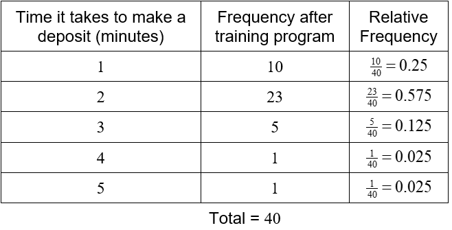
Make a relative frequency table for the time it takes to make a deposit after the training program.
Solution The data values are the deposit times. To create the relative frequencies, divide each frequency by the sum of the frequencies.
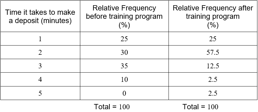
The relative frequency table allows us to see how frequently each data value occurs. For this purpose, the relative frequency may be written as a percentage instead of a decimal. This is done by multiplying the decimal by 100. This means that the totals in each column will be 100 instead of 1.
From the relative frequencies, we see that deposits taking 3 or 4 minutes prior to the training program are reduced after the training program. This results in an increase in deposits taking 2 minutes. In fact, deposits taking 2 minutes or less increased from 55% of deposits (25 + 35) to 82.5% (25 + 57.5) of deposits.
The time it takes to make a deposit is an example of quantitative data. This means that the data value is a number. In this case, the data values were times in minutes. A relative frequency table may also be computed using qualitative data. Qualitative data describes some attribute of an occurrence.
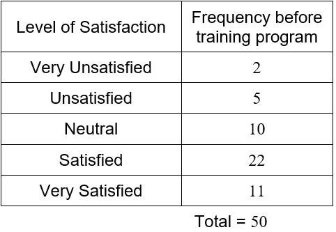
Suppose a customer satisfaction survey is administered to the customers exiting the bank. The survey asks the customer to rate their satisfaction with their visit as very satisfied, satisfied, neutral, unsatisfied, or very unsatisfied. Based on this survey, the following frequencies are calculated.
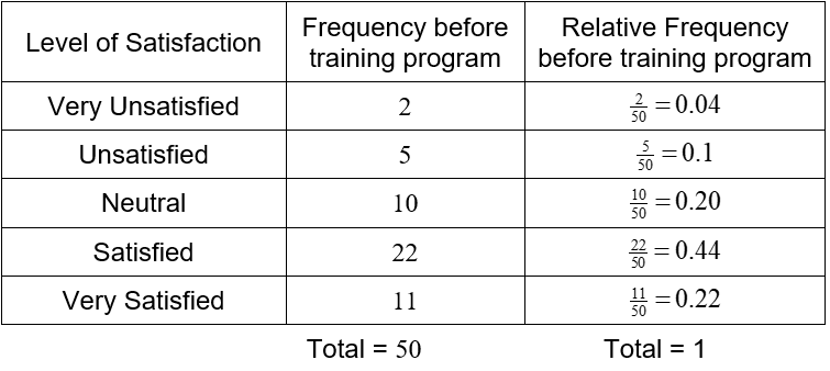
The sum of the frequencies is higher since the survey also encompasses customers who utilized services other than making a deposit. Even though the data are not numbers, we can still use the frequencies to compute relative frequencies.
Example 3 Find a Relative Frequency Table
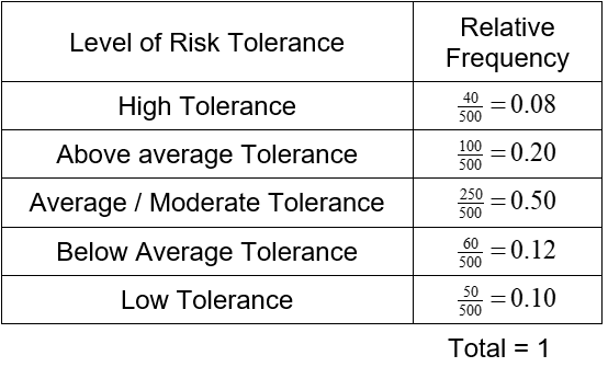
An investment firm administers a survey to its clients to determine their risk tolerance. Based on this survey, the firm puts each of their 500 clients into one of five categories. The table below reflects these results.
Make a relative frequency table for this data.
Solution For each level of risk tolerance, divide the frequency by the total number of clients. This give the following relative frequency table.
A variable that only takes on a finite number of values is called a discrete variable. In each of the previous examples, the number of possible data values for the variable was small. This meant the frequency tables only needed a few rows. If a variable takes on many values, we need additional rows corresponding to each value the variable may take.
Continuous variables may take on any value over an interval. Examples of this type of variable are weight and length. If we were to make a frequency distribution for a continuous variable, the table could potentially have a huge number of rows since every data value might be different.
Discrete variables with many different data values or continuous variables may be displayed in a meaningful way using a grouped frequency distribution. In this type of frequency distribution, each data value is sorted in a category or class. This allows us to calculate the frequency which data values fall into the class.
Let’s look at a concrete example.
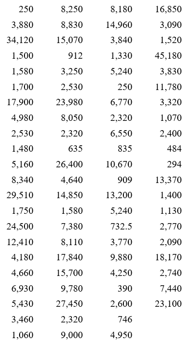
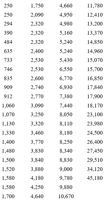
The table above corresponds the market capitalization (in millions of dollars) of 86 companies in the energy sector of the New York Stock Exchange on July 7, 2012. The market capitalization of a company is the value of all shares for the company.
To create a grouped frequency distribution, we start by sorting the data from smallest to largest.
This sorted list, called a data array, shows the smallest market capitalization in the upper left. The market capitalization increases as you move down and to the right in the table.
Now we must define the classes to which each of these data should be placed in. The classes must be defined so that each data value falls into only one of the classes. For these companies, the market capitalizations all fall from 250 through 45,180. This means that the values cover a range of values 45,180 – 250 or 44930 wide. In general, we use between 5 and 15 classes. If possible, we also use classes that are of equal width to make it easier to compare relative frequencies.
Let’s try 8 classes for this data. Each class must have a width of about 44930/3 . This is not a very nice number so we round up to the next convenient value like 6000.
We could start at 250 with classes that are 6000 wide. However, if we start at 0 and use eight classes that are 6000 wide we will include all of the data values.
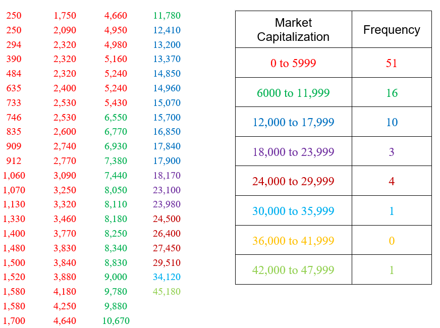
The classes above do not overlap and insure that each data value will fall into one of the classes. The second number in each class is chosen carefully to insure the classes contain all data values. In this case, each value is rounded to the nearest integer when calculating the frequency. If all of the data had been written to the hundredths place, we would also want to write the classes to the nearest hundredth. Now we’ll scan the table and calculate the frequency for each class.
We have color coded the appropriate numbers in the table to make them easier to count. Strategies like this help to insure that all values are accounted for and put into the correct class.
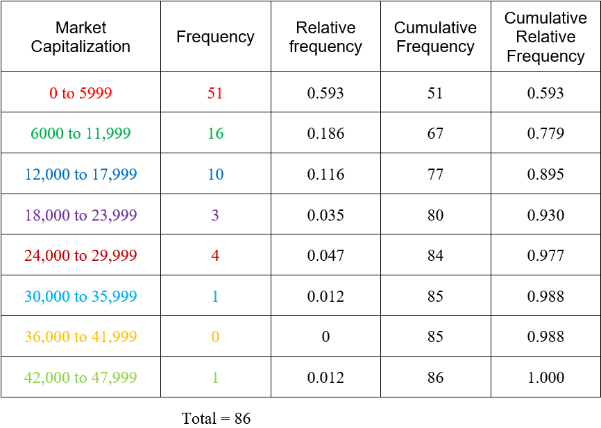
Once we have the frequencies, we can calculate the relative frequencies.
Due to rounding, the sum of the relative frequencies exceed 1 by a small amount. This table also includes the cumulative and cumulative relative frequency. The cumulative frequency of a class is the number of data values that are less than the upper boundary of the class. For instance, the cumulative frequency for the market capitalization from 12,000 to 17,999 is the number of companies whose market capitalization is 17,999 or less. This frequency is simply the sum of the frequencies for the class from 12,000 to 17,999 and all of the frequencies for the classes below it or 51 +16 + 10 = 77. The cumulative relative frequency is found by dividing the cumulative frequency by the total. For the class from 12,000 to 17,999, this gives us 77/85 ≈ 0.895. This tells us that approximately 89.5% of the companies have a market capitalization of 17,999 million dollars or less.
Example 4 Grouped Data
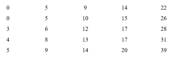
The manager at a bank monitors the amount of time a customer spends in line waiting for a teller. They record this value, in seconds, for 25 customers on a Friday afternoon.
a. Use this data to make a table that includes a column for the relative frequency and the cumulative relative frequency. Use 6 classes to group the data.
Solution Start by putting the data in order.
The class width is
We will round up to a width of 7 and sort the data into the classes below. These classes include all times in the data and do not overlap.
In this table the relative frequencies are calculated by dividing the frequencies by 25. The cumulative frequencies are determined by finding the wait times that are below the upper limit in the class.
b. What proportion of the wait times are at least 14 seconds, but less than 21 seconds?
Solution The relative frequency for the class from 14 seconds to under 21 seconds is the proportion of wait times in the class 14 to under 21:
This means 24 percent of the wait times are 14 minutes to under 21 minutes.
c. What proportion of the wait times are less than 21 seconds?
Solution The cumulative relative frequency for the class from 14 to under 21 minutes is the proportion of wait times less than 21 minutes:
This means 80 percent of the wait times are less than 21 minutes.
