
“Detroit Science Center” by John Kannenberg is licensed under CC BY-NC-ND 2.0
You have probably heard of the “bell” curve, but you may not be familiar with what is really is. Some students may ask their instructors, “Do you grade on a curve?” Before you ask that question, make sure you understand what it is and whether it may be to your advantage.
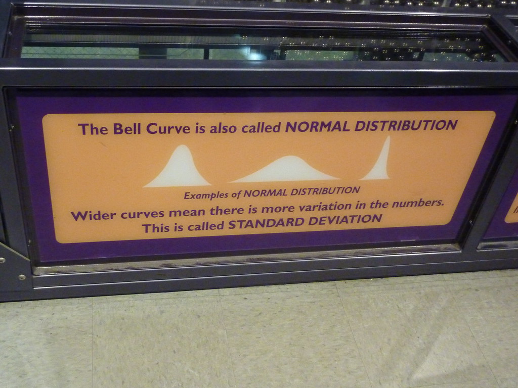
The normal distribution (or bell curve) refers to a histogram that looks like the graphic above. It indicates how data is distributed with respect to each other. As you might guess, the peak of the curve corresponds to the mean and its spread matches the standard deviation.
In this section, you learn about the normal distribution and how to apply it to everyday problems. Our objectives are to
- describe the basic properties of the normal distribution,
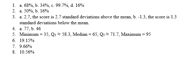
- apply the 68-95-99.7 rule to a set of data,
- relate the area under a normal curve to z-scores,
- convert between raw scores and z-scores, use z-scores to compare data.
Armed with this information, you can utilize the normal distribution to answer questions about the relationship of a specific data value to the data values as a whole.
Use the workbook and videos below to help you master these objectives. Make sure you go through the practice problems since they are reflective of the types of problems you might find on a quiz or exam.
Section 1.6 Workbook on the Normal Distribution (PDF) (7-31-19)
Section 1.6 Practice Solutions
Chapter 1 Practice Solutions (PDF)(9-17-19)
Videos by Mathispower4u by James Sousa is licensed under a Creative Commons Attribution-ShareAlike 3.0 Unported License.

In the video below, think of probability of a data value as meaning the percentage of data values. We are using a cumulative from the mean table in our class (the second one in the video)