
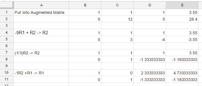
When carrying out row operations in Google Sheets, you may end up with cells whose entries are very long (repeating?) decimals. If you round these numbers, you are potentially changing the solution to the problem you are doing. It would be nice to be able to show the numbers in the lower right hand portion of the picture above as fractions.
Luckily this is possible by formatting those cells with a custom format. To do this, drag select the cells you want to format this way. With the cells selected, go to the Format menu and choose Number.
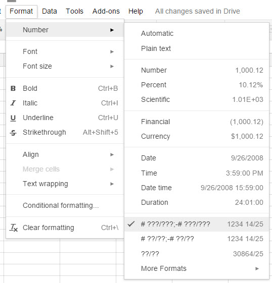
At the bottom of the this menu is submenu called More Formats. When you choose that option, another menu will appear.
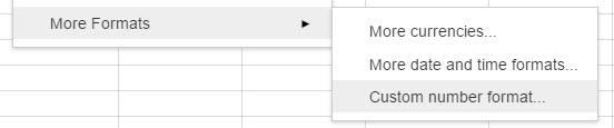
Choose Custom Number Format. This will open a box in which you can customize how the number appears in the cell.
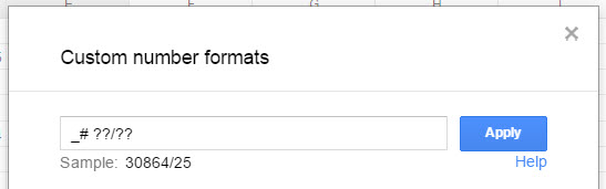
Enter the characters shown above and then press Apply. Make sure the characters start with an underscore ( _ ) and contain a space between the # and the ?.
All of the numbers in the selection will now be written as fractions.
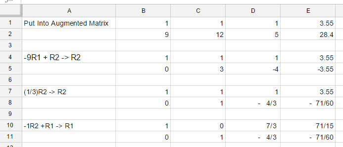
A quick spot check show that cell D8 had contained the decimal -1.333333333. With the new formatting, it appears as the fraction -4/3.
By using the fraction in your solution, you can avoid rounding until the very last step of the calculation where it is more appropriate to round.