How Do You Estimate a Derivative at a Point vs Compute a Derivative at a Point from the Limit?

We are now in the real meat of calculus….rates and derivatives. Essentially, rates are simply slopes. Depending on the field you are working in or the representation of the data or function, it might have a different terminology. Keeping all of these straight is the biggest challenge in the class. Let’s try to put what we know into a table.

Common Description Graphical Interpretation Mathematical Terminology
Average Rate of Change of f(x) from x=a to x=b Slope between (a,f(a)) and (b,f(b))  Slope of the Secant Line from x=a to x=b
 Instantaneous Rate of Change of f(x) at x=a  Slope between (a,f(a)) and (a+h,f(a+h)) where h is very small  Slope of the Tangent Line on f(x) at x=a


If it feels like we use slope to calculate everything…you are right. The only difference is where the two points are located. If they are located fairly far apart, then we are calculating an average rate of change. If they are located an infinitesimal amount apart, then we are calculating the instantaneous rate of change.

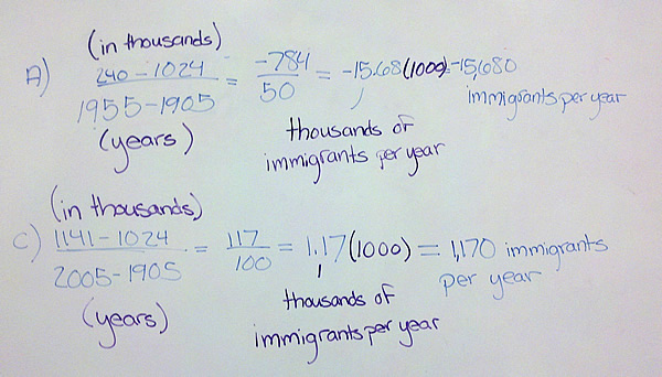
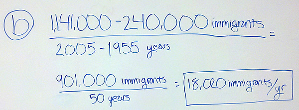
But here is where it gets hazy…if the representation of the function does not allow us to pick the points infinitely close together, we may approximate the instantaneous rate of change with an average rate of change between two points that are as close as the representation allows. I think this point is bothering many of you. It occurs most often when we try to find the instantaneous rate from a data table. In that case, the points are where they are at and we can pick pairs that are closer and closer together. We pick them as close as we can near the place we want the instantaneous rate of change and say we are estimating the instantaneous rate of change.

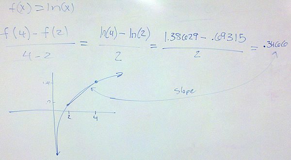
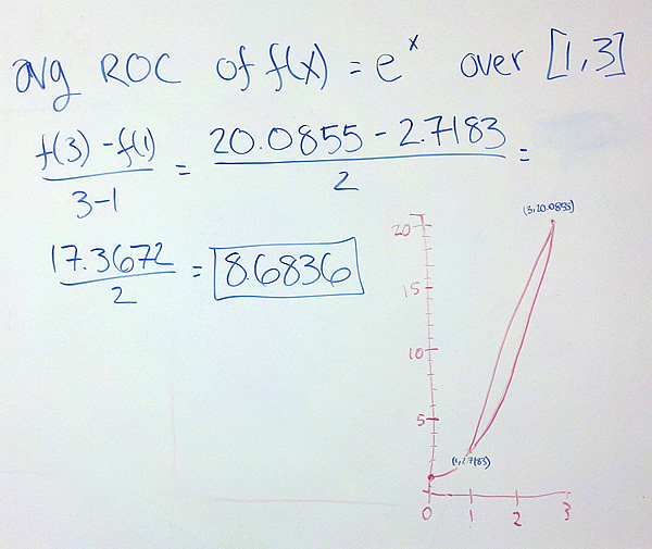
If we are given a graph, we can draw a secant line between the points to calculate the average rate of change. The only estimating done in this case is estimating where the points are on the graph. Our eyes are only so good in reading off the values. For the instantaneous rate of change, we draw the tangent line where we want the rate and eyeball its slope. Again, since we are making educated guesses about the slopes, the numbers are estimates based on our ability to read the slope.

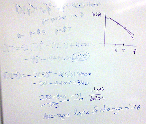
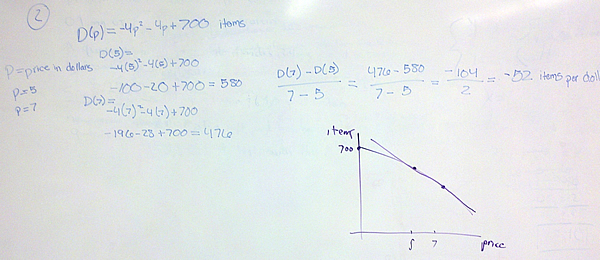
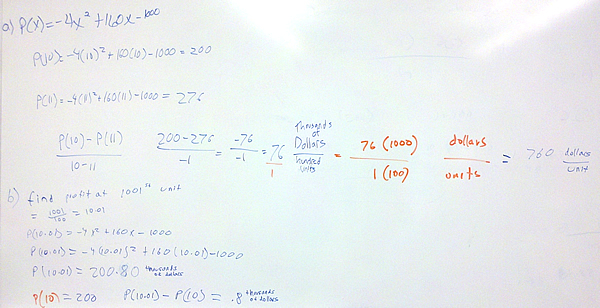
If we are given the function’s formula, we can calculate the average rate or the instantaneous rate exactly. For the average rate of change of f(x) over x = a to x = b, we calculate [latex]{{f(b) – f(a)} \over {b – a}}[/latex].

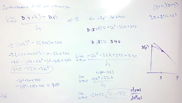
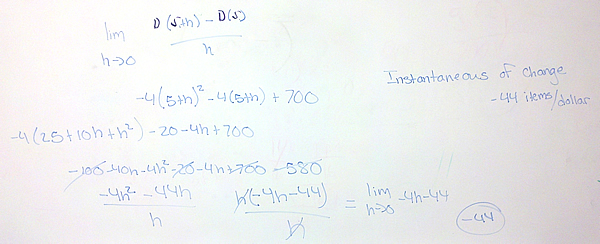
For the instantaneous rate of change, we use the function’s formula to calculate the limit [latex]\mathop {lim }\limits_{h \to 0} {{f(a + h) – f(a)} \over h}[/latex].

The estimating comes from the fact that we may not be able to find two points infinitesimally close or the fact that we cannot calculate the slope perfectly from how the function is given to us.

Another cautionary note…different disciplines call the derivative by different names. Mathematicians call it the derivative of course, but in physics it might be called the instantaneous rate. In finance and economics, it will be called the marginal function. And in other fields you’ll here other terms.

How Do You Find the Average Rate of Change from a Table?

One of the problems on the homework gave you three points on a line graph, (1905, 1024), (1955, 240), (2005, 1141). In these ordered pairs, the x value is the year and the y value is the number of immigrants (in thousands) to a large country.

  1. Find the average rate of change in immigration from 1905 to 1955 in immigrants per year.
  2. Find the average rate of change in immigration from 1955 to 2005 in immigrants per year.
  3. Find the average rate of change in immigration from 1905 to 2005 in immigrants per year.

This problem illustrates the two ways that you can work in the “thousands” in the data to give immigrants per year instead of thousands of immigrants per year.

How Do You Find the Average Rate of Change From a Function?

Problem 1 Find the average rate of change of $latex \displaystyle f(x)=ln (x)$ over [2, 4] to four decimal places.

Problem 2 Find the average rate of change of $latex \displaystyle f(x)= {e}^{x}$ over [1, 3] to four decimal places.

When you calculate the rate to four decimal places, you should write the numbers in the quotient to FIVE decimal places to make sure there are no rounding errors.

How Do You Find the Average Rate of Change From an Econ Formula?

Here are several examples where the average rate of change is calculated from some type of economics formula.

Problem 1 The demand for a particular product is given by

$latex \displaystyle D(p)=-2{{p}^{2}}-2p+400\quad \text{items}$

where p is the unit price in dollars.

a. Find the average rate of change of demand with respect to price between a price of 5 dollars and 7 dollars.

b. Find the instantaneous rate of change of demand at a price of 5 dollars.

(Sorry for the shaky cam…too much caffeine!)

The average rate tells us that for each increase in price of 1 dollars between 5 dollars and 7 dollars, the demand for the product drops by 26 items. The instantaneous rate of change tells us that at a price of 5 dollars, the demand is dropping by 22 items per dollar.

Problem 2 The demand for a particular product is given by

$latex \displaystyle D(p)=-4{{p}^{2}}-4p+700\quad \text{items}$

where p is the unit price in dollars.

a. Find the average rate of change of demand with respect to price between a price of 5 dollars and 7 dollars.

b. Find the instantaneous rate of change of demand at a price of 5 dollars.

Problem 3 The profit (in thousands of dollars) for selling x hundred units of compressors is

$latex \displaystyle P(x)=-4{{x}^{2}}+160x-1000$

a. Find the average rate of change of profit with respect to compressors from x = 10 to x = 11.

b. Find the exact profit from the 1001st compressor.

c. Find the instantaneous rate of change of profit with respect to compressors at x = 10.

Problem 4 The profit (in thousands of dollars) for selling x hundred units of graphics displays is

$latex \displaystyle P(x)=-5{{x}^{2}}+80x-100$

a. Find the average rate of change of profit with respect to displays from x = 10 to x = 11.

b. Find the exact profit from the 1001st display.

c. Find the instantaneous rate of change of profit with respect to displays at x = 10.

In these last two problems, pay careful attention to the units on the rates. They are all in thousands of dollars per hundred units. This simplifies to tens of dollars per unit since one thousand divided by one hundred is ten.

Also note that to find the profit from the 1001st item, we need to find the profit at a production level of 1001 and subtract the profit at a production level of 1000. This quantity is called the marginal profit at a production level of 1000. As noted in the text, it is approximately equal to the instantaneous rate of change at a production level of 1000.