
A matrix is entered between curly brackets in WolframAlpha (http://www.wolframalpha.com). Additionally, each row of the matrix is entered in curly brackets too.
You can also put a matrix in reduced row echelon form. We could put the augmented matrix
$latex \displaystyle \left[ \begin{array}{*{35}{l}}
1 & 2 & -1 \\
4 & 3 & 1 \\
\end{array} \right]$
Use the text “row reduce” and then enter the matrix. The solution is x = 1 and y = -1.
Let’s try this with another system of linear equations
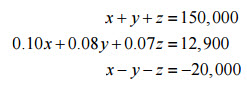
Convert this system into a 3 x 4 augmented matrix:
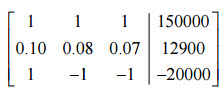
WolframAlpha understands several commands for putting an augmented matrix into reduced row echelon form. You can use the command rref { }or the command row reduce { }. The matrix goes inside the curly brackets. However, the matrix must be put in carefully. Each row needs to be typed in inside of curly brackets with the entries separated by a commas. In this case, you would type
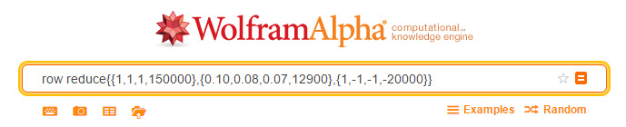
on the command line in WolframAlpha.
After you press Enter, the reduced row echelon form is computed,
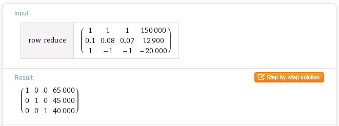
This indicates that the solution to the system is
x = 65,000, y = 45,000, z = 40,000.
