Working with frequency distributions to find the mean, variance, and standard deviation can be a little tough. In the example below, we’ll incorporate Sheets (or Excel) to make it easier to calculate these statistics. An example is worked out in Example 3 of Question 2 in Section 6.2 for the mean and in the video below for standard deviation.
Let’s look at how we can implement this process in a spreadsheet.
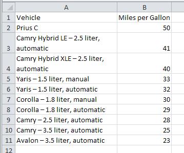
In 2012, Toyota claimed to have the most fuel efficient passenger car fleet. Based on mileage estimates from Edmunds.com, the table below shows the mileage of passenger vehicles manufactured by Toyota.
Vehicle
Miles per Gallon
Prius C
50
Camry Hybrid LE – 2.5 liter, automatic
41
Camry Hybrid XLE – 2.5 liter, automatic
40
Yaris – 1.5 liter, manual
33
Yaris – 1.5 liter, automatic
32
Corolla – 1.8 liter, manual
30
Corolla – 1.8 liter, automatic
29
Camry – 2.5 liter, automatic
28
Camry – 3.5 liter, automatic
25
Avalon – 3.5 liter, automatic
23
Use this table to find the mean miles per gallon for Toyota passenger vehicles in 2012.
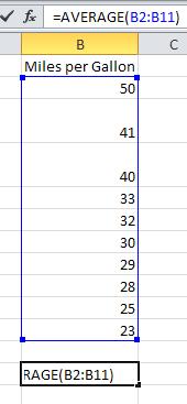
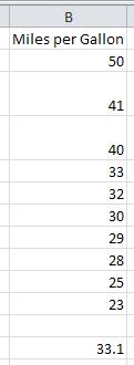
Solution To find the mean using Excel, we’ll use the spreadsheet command AVERAGE.
1. Enter the data from the table into the different cells in the spreadsheet. Column A is not required, but is useful.
2. Click on cell B13. This is where we will place the mean of the data. Type =AVERAGE( as shown to the right. The command will be shown in the cell as well as the function bar. To indicate the location of the data, type B2:B11. You can also click in cell B2, hold the left mouse button down and drag the cursor to cell B11. Type ) to complete the command.
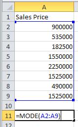
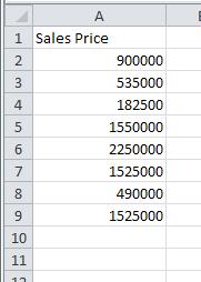
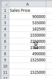
During the week of 6/7/2012 through 6/14/2012, eight homes were sold in Paradise Valley, Arizona in the area code 85253. The sales prices for these homes are listed below.
Solution Use the MODE command in a spreadsheet to compute the mode of the data.
1. Enter the data from the table into the different cells in a spreadsheet.
2. Click on cell A11. This is where we will place the mode of the data. Type =MODE( as shown to the right. The command will be shown in the cell as well as the function bar. To indicate the location of the data, type A2:A9. You can also click in cell A2, hold the left mouse button down and drag the cursor to cell A9.

 Working with frequency distributions to find the mean, variance, and standard deviation can be a little tough. In the example below, we’ll incorporate Sheets (or Excel) to make it easier to calculate these statistics. An example is worked out in Example 3 of Question 2 in Section 6.2 for the mean and in the video below for standard deviation.