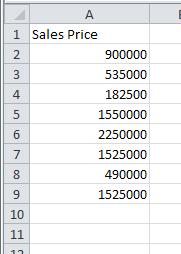
During the week of 6/7/2012 through 6/14/2012, eight homes were sold in Paradise Valley, Arizona in the area code 85253. The sales prices for these homes are listed below.
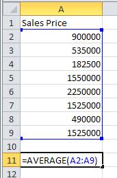
Solution Use the AVERAGE command to compute the mean of the data.
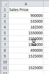
Enter the data from the table into the different cells in a spreadsheet.
2. Click on cell A11. This is where we will place the mean of the data. Type =AVERAGE( as shown to the right. The command will be shown in the cell as well as the function bar. To indicate the location of the data, type A2:A9. You can also click in cell A2, hold the left mouse button down and drag the cursor to cell A9. Type ) to complete the command.
Press Enter to compute the mean. In cell B11, type Mean to identify the type of central tendency.
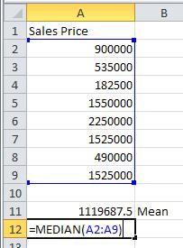
b. Find the median sales price.
Solution Use the MEDIAN command to compute the median of the data.
In cell A12, type =MEDIAN(A2:A9).
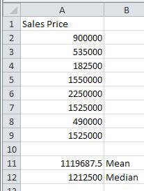
3. Press Enter to compute the median.
4. In cell B12, type Median to identify the measure of central tendency.
During the week of 6/7/2012 through 6/14/2012, eight homes were sold in Paradise Valley, Arizona in the area code 85253. The sales prices for these homes are listed below.
Solution Use the MODE command in a spreadsheet to compute the mode of the data.
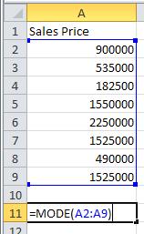
1. Enter the data from the table into the different cells in a spreadsheet.
2. Click on cell A11. This is where we will place the mode of the data. Type =MODE( as shown to the right. The command will be shown in the cell as well as the function bar. To indicate the location of the data, type A2:A9. You can also click in cell A2, hold the left mouse button down and drag the cursor to cell A9.
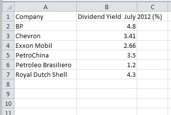
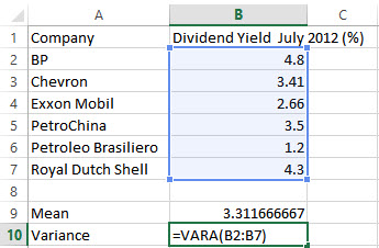
The table below shows the dividend yields of six companies in the New York Stock Exchange energy sector.
Company
Dividend Yield July 2012 (%)
BP
4.80
Chevron
3.41
Exxon Mobil
2.66
PetroChina
3.50
Petroleo Brasiliero
1.20
Royal Dutch Shell
4.30
a. Find the sample mean.
Solution Use the AVERAGE command in a spreadsheet to compute the mean.
1. Enter the data from the table into the different cells in the spreadsheet.
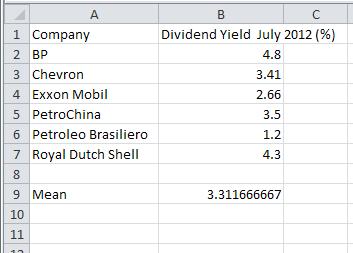
2. In cell A9, type Mean to indicate that the number in B9 will be the mean.
3. Click on cell B9. This is where we will place the mean of the data. Type =AVERAGE( as shown to the right. To indicate the location of the data, type B2:B7. You can also click in cell B2, hold the left mouse button down and drag the cursor to cell B7. Type ) to complete the command.
4. Press Enter to compute the mean.
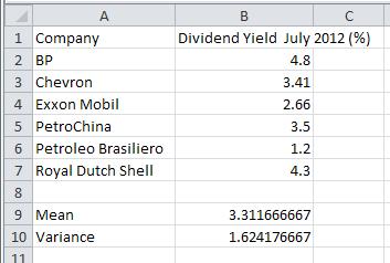
b. Find the sample variance.
Solution Use the VARA (VARPA for population variance) command to compute the sample variance of the data.
1. Type Variance in cell A10. Since we need the sample variance, type =VARA( in cell B10. Type B2:B7 or drag select these cells to identify the location of the data.
2. Press Enter to compute the sample variance.
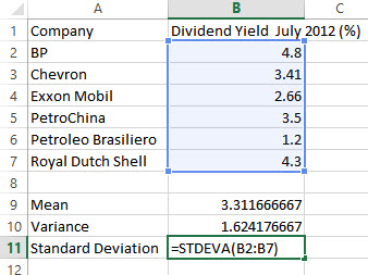
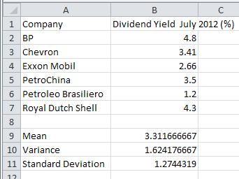
c. Find the sample standard deviation.
Solution Use the STDEVA command to find the sample standard deviation of the data.
1. In cell A11, type Standard Deviation. In cell B11, type STDEVA( . Type B2:B7 or drag select these cells to identify the location of the data. To compute the population standard deviation, you would use the command STDEVPA. Type ) to complete the command.
2. Press Enter to compute the sample standard deviation.
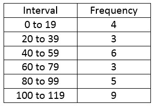
Suppose we are given some frequencies corresponding to some data in intervals.
To find the mean, we need to find a representative data value from each interval.
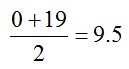
We’ll use the midpoint of each interval. The midpoint for the first interval is
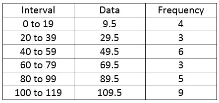
We can find the other midpoints in a similar manner. Let’s add this to the table.
Let’s put this information in a spreadsheet.
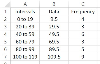
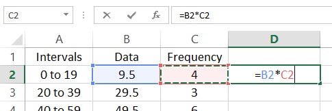
To find the mean of this frequency distribution, multiply each data value times its corresponding frequency. In the spreadsheet, put =B2*C2 in cell D2.
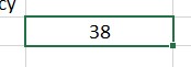
Press Enter to compute this value. Next we need to fill this value into the cells D3 through D7. Click on cell D2. The cell will be outlined like you see below.
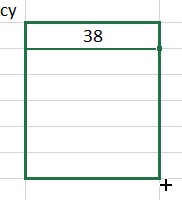
Place your mouse over the box in the lower right hand corner of this outline. The cursor will change to a black cross. Hold down the left mouse button and drag the cursor to cell D7.
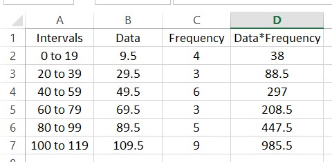
When you release the button, the products will be calculated for each row. Adding a label in cell D1 might help you to remember what the numbers in the cell are.
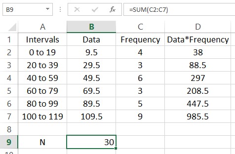
The function SUM is useful for adding up lists of numbers. For instance, we can find the sum of the frequencies N by typing =SUM(C2:C7). Put this formula in cell B9.
In this picture a label has been added in A9 to help the reader understand what is in the cell to the right. Add another label in cell A10 with the text “Mean”. Next to that cell we’ll calculate the mean of the data. This is done by adding the entries in column D and dividing by the sum of the frequencies in cell B9.
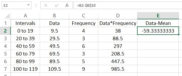
Finding the variance is a bit more complicated. In this calculation we need to subtract the mean from each data value and square the result. This needs to be done with an absolute reference to cell B10 so that the fill always refer to that cell in making the calculation. Start by clicking in cell E2 and typing =B2-$B$10.
This means that the data value 9.5 is approximately 59.3 units below the mean. Fill the rest of the column and we end up with this worksheet.
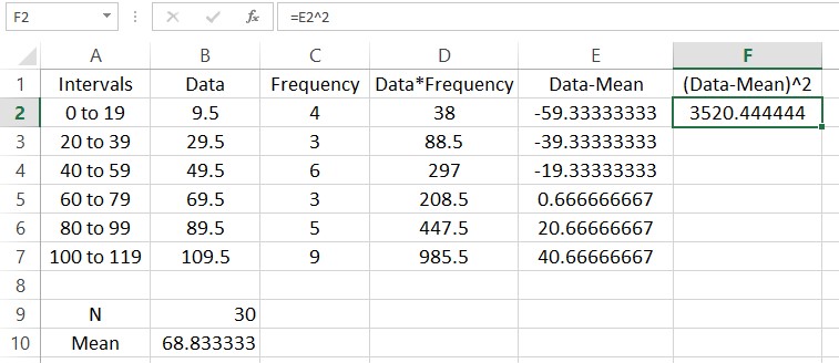
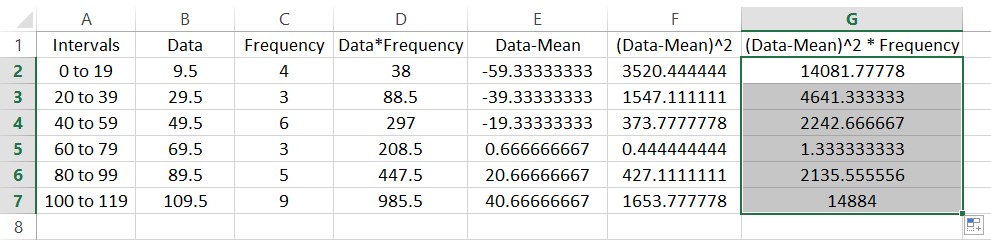
We could sum these deviation now, but the positive and negative nature of each row would mask the spread of the data. Squaring each of the entries makes each of them positive. In cell F2, type =E2^2.
Fill the rest the rows using a fill.
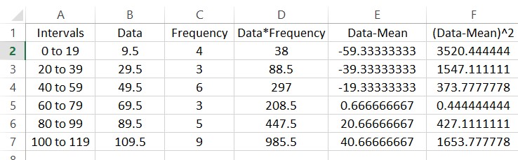
The entries in this column are often called the deviations from the mean squared. Each of these occur with the frequencies in column C. To find the sample variance, multiply the entries in column F by the frequencies in column C to give the worksheet below.
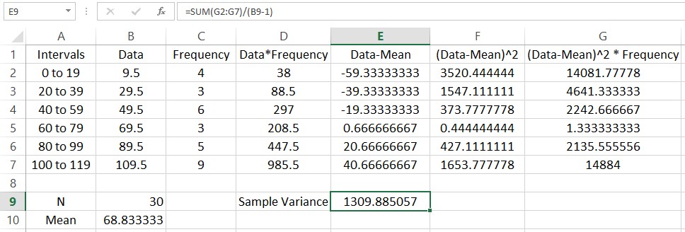
Let’s calculate the variance. Start by typing a label for the sample variance in cell D9. In the adjacent cell we’ll put the value. The variance is the sum of the entries divided by the sum of the frequencies minus 1. In cell E9, type =SUM(G2:G7)/(B9-1).
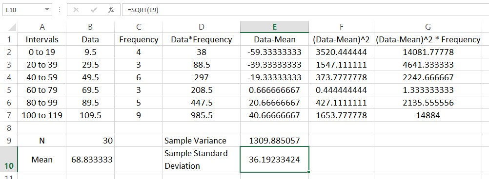
The sample standard deviation is the square root of the standard variance. We can take the square root using the function SQRT. Put a label in cell D10 and type =SQRT(E9) in the adjacent cell.
The standard deviation is a measure of how spread out the frequency distribution is around the mean.
In your classes, you might hear about instructors who grade on “a curve”. There is an idea that this might somehow benefit you when it comes to grading. Let’s take a look how that might work if the curve is a normal curve.
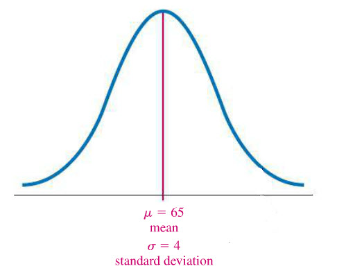
Problem Suppose you and your classmates take an exam that has a mean of 65 and a standard deviation of 4. If the instructor says the top 10% of scores earns an A, what is the cutoff for an A?
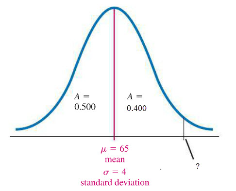
Solution Pictorially, the frequency distribution look like the bell curve below.
We know that 50% of the test score lie on the left side of the mean so the area on the left side of the mean and under the bell curve is 0.5. Now let’s label a point on the right hand side of the mean where 40% of the scores are from the mean to that point.
At the point labeled by ?, 90% of all scores are below this point (or 10% of scores are above this point).
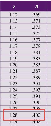
We can locate this point using a table of z-scores and areas. Look for the z score that corresponds to an area of A = 0.4.
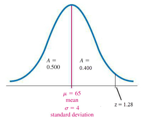
Examining the data, we see that this corresponds to a z-score of 1.28.
But what is the data or raw score that corresponds to a z-score of 1.28?
To find this data value, start with the formula for z-scores,
And put in the values:
To solve for the data value x, multiply both sides by 4 and then add 65 to both sides.
This tells us that 90% of scores lie below 75.12 and 10% of the scores are above 75.12. To earn an A, you would need to score greater than 75.12.