Category: Finite Mathematics Ebook

How do you get the optimal solution to a standard maximization problem with the Simplex Method?

In the previous question, we learned how to make different variables into basic and nonbasic variables. This allowed us to calculate the locations of corner points on the feasible region and other points of intersection. For simple linear programming problems, there can be many such points. If we naively make different variables into basic variables, it may take a very long time to find the corner point that optimizes the objective function.

The Simplex Method is an algorithm for solving standard maximization problems. By following the steps below, you ensure that the points you find by changing basic variables are corner points of the feasible region. In addition, the algorithm is iterative. In other words, it is carried out several times with the result of each iteration providing the starting point to the next iteration. The beauty of the Simplex Method is that each iteration yields a larger value for the objective function and eventually leads to the largest possible value for the objective function.

To get a feel for how the Simplex Method works, let’s solve the standard maximization problem

We’ll start by converting this problem to an appropriate system of linear equations. Add a different slack variable to each constraint to yield

To convert the objective function to an appropriate form, move all of the terms with variables to the left side of the equation. This is done by subtracting 5x and 6y from both sides. This yields the equation -5x -6y + z = 0.

These equations form the system of linear equations

The augmented matrix for this system,

is the initial simplex tableau. It is the starting point for carrying out the Simplex Method algorithm. The bottom row of the tableau is called the indicator row. The algorithm starts by determining which variable will become a basic variable in the first iteration of the algorithm. The variable that corresponds to the most negative entry in the indicator row will become a basic variable.

For this matrix, the most negative entry is -6 in the second column. The variable y that corresponds to the column will become the basic variable. This column is the pivot column.

If we pick the column with the most negative entry in the indicator row to be the pivot column, the objective function will increase by the largest amount. Remember, those negative entries correspond to positive coefficients in the original objective function. For the objective function z = 5x + 6y, the most negative entry in the indicator row, -6, corresponds to the largest positive coefficient, 6, in the objective function. Increasing the value of y in the potential solution from 0 to some positive value leads to a larger increase in the objective function value z than increasing the value of x from 0 to the same positive value. This is due to the fact that the coefficient on y is larger than the coefficient of x. In effect, it is more efficient to change y values than x values in the solution.

We know that we’ll need to make all of the entries but one in that column equal to zero via row operations. The other entry will be a one. The row where we will put the one is called the pivot row, and the entry that becomes a one is called the pivot. To find which row will become the pivot row, we form quotients from the entries in the pivot column and the last column:

The row whose quotient is positive and smallest is the pivot row. In this case, the second row is the pivot row so the pivot is the number 2 in this row.

As we saw earlier, picking the pivot row carefully guarantees that the potential solution stays in the feasible region and all variables are non-negative. The variables must remain non-negative for a standard linear programming problem.

Let’s look at this idea more closely. Look at the initial tableau from the standard linear programming problem:

We already know that y will become a basic variable based on the numbers in the indicator row. By making y a basic variable, either s₁ or s₂ will join x as a nonbasic variable. The question is, which will it be?

Suppose that s₁ and x will be the nonbasic variables in the next tableau, and will be set equal to zero. In this case, we can use the first row of the tableau to determine the corresponding value of y:

The value of s₂ is found from the second row of the tableau by setting the nonbasic variables equal to zero and y = 4:

This is not a reasonable solution since the slack variable s₂ is negative.

Let’s look at making s₂ and x the nonbasic variables. In this case, we can use the second row of the tableau to determine the corresponding value of y:

The value of s₁ is found from the first row of the tableau,

All variables in this case are non-negative. Note that the values for y in each case are precisely the quotients we use to choose which row becomes the pivot row. By choosing a value for y that is smaller (the smaller quotient), we get a situation in which all variables are non-negative.

Now that we know that the pivot is the 2 in the second row, second column of

we’ll use row operations to change it to a 1. The rest of the pivot column will be changed to zeros using row operations. This change in basic variables will lead to the largest increase in the value of the objective function and keep all variables non-negative.

As shown in Question 3, change the pivot to a one by multiplying the second row by ¹/₂:

Once the pivot is in place, use row operations to place zeros in the rest of the column:

In the Simplex Method, the optimal solution is obtained when there are no negative numbers in the indicator row.

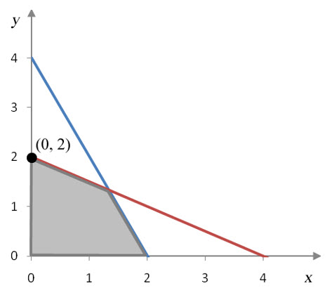
Since the transformed matrix has a negative number in the indicator row, the solution (x, y) = (0, 2) is not optimal. The value of the objective function, z = 12, can be made greater by picking the first column to be the pivot column. To find the pivot row, examine the quotients formed from dividing entries in the last column by corresponding entries in the pivot column:

The smallest quotient is ⁴/₃ in the first row. The pivot, ³/₂, is in the first row, first column. As in the first iteration, we must use row operations to change the pivot to a one and change the rest of the pivot column to zeros.

To change the pivot to a one, multiply the first row by ²/₃:

To complete the transformation of the pivot column, we must use row operations to put zeros in the rest of the pivot column:

For this tableau, the basic variables are x, y, and z. The nonbasic variables are s₁ and s₂. The indicator row has no negative entries so this tableau is the final tableau. The optimal solution is read from this tableau by setting the nonbasic variables equal to zero.

If we cover the nonbasic variables,

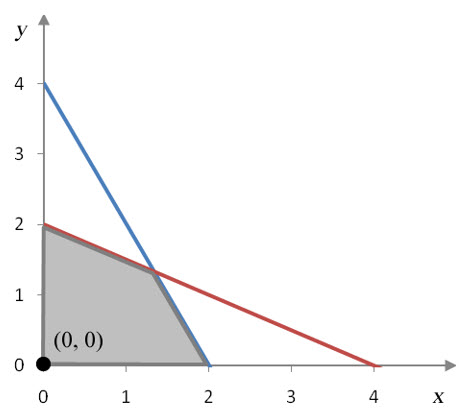
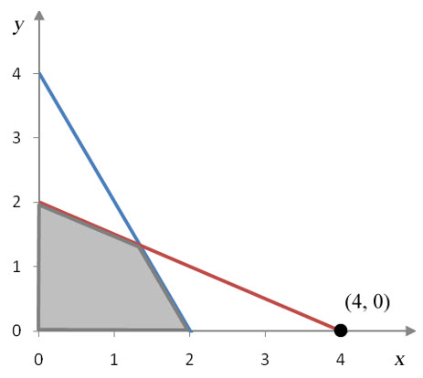
we see that this tableau corresponds to (x, y) = (⁴/₃, ⁴/₃) and an optimal value of z = ⁴⁴/₃. This is the same value we found graphically in Section 4.2

The process outlined here is summarized in the steps shown here.

The Simplex Method will reach an optimal solution for a standard maximization problem with any number of variables and any number of inequalities. However, problems with large numbers of variables and inequalities may require many iterations of steps 5 through 9 to reach the optimal solution. Take special care to avoid arithmetic errors when carrying out the row operations. A graphing calculator or spreadsheet can make the task of carrying out the row operations fairly painless.

Example 3    Find the Optimal Solution

Find the optimal solution to the linear programming problem

Solution Although this example has three constraints (in addition to the non-negativity constraints), it still has two decision variables. Each constraint needs a slack variable to convert it to an equation. Using the slack variables s₁, s₂, and s₃, the constraints become

Move all of the variable terms in the objective function to the left side of the equation to yield

These equations become the initial simplex tableau

The bottom row of the initial simplex tableau is the indicator row. The most negative entry of the indicator row is -5. This means the pivot column is the second column in the tableau.

To determine the pivot row, compute the quotients formed by dividing entries in the last column by entries in the pivot column,

Any negative quotients, such as –³/₅ in the third row, are discarded. The quotient formed in the first row, ¹⁵/₃, is the smallest quotient so the pivot is the 3 in the first row, second column.

In the first iteration of the simplex method, we must use row operations to change the pivot to a one and all other entries in the pivot column to zero.

The pivot is changed to a 1 by multiplying the first row by ¹/₃. Carrying out the row operation yields

Three row operations are necessary to put the zeros in the rest of the pivot column:

The new tableau corresponds to the solution (x₁, x₂) = 0, 5) and is not optimal since there is a negative entry in the indicator row.

The new pivot column is the first column due to the negative number in the indicator row. To find the new pivot row, compute the quotient formed from dividing the entries in the last column by the entries in the new pivot column:

The second row is the only row with a valid quotient so it is the pivot row. The pivot is the 11 in the second row, first column of the tableau.

Multiply the pivot row by ¹/₁₁ to change the pivot to a 1:

To complete this Simplex Method iteration, we must place zero above and below the pivot using row operations.

Three row operations are required to place the zeros above and below the pivot.

The indicator row does not contain any negative numbers so the optimal solution has been reached.

The solution to the linear programming problem is easily observed by covering the columns corresponding to the nonbasic variables s₁ and s₂:

The optimal solution to the linear programming problem is z = 29 and occurs at (x₁, x₂) = (3, 7).

How do you find a basic feasible solution?

The initial simplex tableau allows us to calculate the locations of the corner points as well as any other points where the lines corresponding to the equations cross or cross the axes. Let’s start with the initial simplex tableau

Since there are more variables than equations, there is not a unique solution to the system of equations represented by the tableau. There are five variables and three equations so we need or 2 parameters to write the solution. Any two of the variables may be parameters, but in the case of the initial simplex tableau it is convenient to choose the parameters as x and y.

To see why, rewrite the augmented matrix as a system of equations,

The variables s₁, s₂, and z each have a coefficient of 1 and appear nowhere else in the system. In the matrix, this corresponds to the columns consisting of all zeros except for a single entry of 1. These variables are the basic variables for the initial simplex tableau. The other variables, x and y, are the nonbasic variables for the initial simplex tableau. To find possible corner points, we’ll solve for the basic variables in term of the nonbasic variables.

Solve for the basic variables variables in terms of x and y:

One possible solution to this system is found by setting the nonbasic variables x and y equal to zero. In this situation,

This situation corresponds to the corner point of the feasible region at (x, y) = (0, 0) with an objective function value of z = 0. At this corner point, the slack variables take on the values s₁ = 4 and s₂ = 4.

Figure 1 – The corner point corresponding to a solution of the initial simplex tableau with s₁ = 4, s₂ = 4 and z = 0.

Other corner points can be obtained by using row operations to make other variables basic instead of s₁, s₂, and z. In general, z should always be a basic variable so that it is easy to determine the value of the objective function.

Suppose we start from the initial simplex tableau

and multiply the second row by ¹/₂ and place the result in the second row (¹/₂ R₂ becomes R₂). This gives us a 1 in the second row, second column:

If we make the rest of the second column zeros, the variable y will become a basic variable. To do this, we’ll use two row operations.

First, multiply the second row by -1 and add it to the first row:

This sum will be placed in the first row. Second, multiply the second row by 6 and add it to the third row:

This sum is placed in the third row. Putting these rows into the tableau yields

In this tableau, the variables y, s₁, and z are basic. The variables x and s₂ are nonbasic variables. Notice that by placing the 1 in the second column in the second row, the second slack variable (which originally was in the second row) became nonbasic. In general, when a 1 is placed in a column to make a variable basic, the slack variable corresponding to the row it was placed in becomes nonbasic. As with the initial simplex tableau, we’ll write this matrix as a system of equations and set the nonbasic variables equal to zero.

The corresponding system of equations is

If we solve each equation for a different basic variable we get

If we set the nonbasic variables x and s₂ equal to zero, we find that s₁ = 2, y = 2, and z = 12. This corresponds to the corner point at (x, y) = (0, 2) with an objective function value of z = 12.

 

Figure 2 – The corner point at (0,2) corresponding to s₁ = 2, y = 2, and z = 12.

It is easier to find this corner point using the tableau without transforming it to a system of equations. The key is to realize that when nonbasic variables are set equal to zero, their coefficients in the matrix disappear. For instance, if we take the tableau we transformed with row operations and cross out the columns of the nonbasic variables we get:

By ignoring these columns, we can see that s₁ = 2, y = 2, and z = 12. Combining this observation with our knowledge of setting the nonbasic variables equal to zero gives us the corner point at (0, 2) and objective function value z = 12.

We cannot arbitrarily make a variable into a basic variable. For instance, we might make x a basic variable by putting a 1 in the second row and first column and zeros in the rest of the column. Starting from the original simplex tableau, we must carry out two row operations:

To find the corner point corresponding to this matrix, cover the nonbasic variables and read off the values of the basic variables:

Figure 3 – A solution to the tableau that is not a corner point of the feasible region.

On the surface this might not seem all that different from earlier tableaus, but this one violates one of the assumptions for slack variables. In a standard maximization problem, the slack variables are assumed to be non-negative. In the solution we found from this tableau, the value for s₁ is negative. This tells us that this solution does not correspond to a corner point of the feasible region.

The solution we have just found, (0, 4), matches a point on a line, but is not along the border of the feasible region. If we are not careful about picking the basic and nonbasic variables, we may obtain a point that is not related to the solution.

If we want to make the variable x a basic variable, it is better to use row operations to transform the original matrix

By covering the columns under y and s₁, we observe that this new tableau corresponds to the solution x = 2 and y = 0 and the objective function value z = 10. This does match the corner point (2, 0) on the feasible region.

Example 2    Change Basic Variables

The basic variables for the initial simplex tableau
are s₁, s₂, and z. Use row operations to change the tableau so that the basic variables are y, s₁, and z. What corner point of the basic feasible solution does this new tableau correspond to?

Solution We want to change the basic variables from s₁, s₂, and z to y, s₁, and z. This means we need to make s₂ nonbasic and y basic. The other two variables, s₁ and z, should remain basic variables.

To make y a basic variable, we need to place two 0’s and a 1 in the column corresponding to y. The only question is where should we put the one? The first row of the second column already has a one so all we need to do is to use row operations to place zeros in the rest of the column.

If you examine the new matrix, you’ll notice that y is a basic variable, but s₁ is not. Instead, s₂ is a basic variable.

If we place the one in the first row, the slack variable corresponding to that row, s₁, becomes a nonbasic variable. Since we want s₁ to remain basic and s₂ to become nonbasic, the one should be placed in the second row of the first column. Start from the original tableau

In general, we get the one by multiplying the row by a constant:

Now we can add multiples of rows to put zeros in the rest of the second column.

Since the second, third, and fifth columns contains two zeros and a one, the basic variables are now y, s₁, and z. The point in the feasible region corresponding to this tableau is found by covering the nonbasic variable columns x and s₂. This shows the corner point to be at with an objective function value of z = 12.

What are slack variables?

The graphical strategy for solving linear programming problems relies on the idea that the maximum value of the objective function will occur at a corner point of a bounded feasible region. The Simplex Method is no different, but we need to work with equations for the border of the feasible region in matrix form. The trouble is that augmented matrices are designed to solve equations and we have inequalities. For the graphical strategy, we simply converted each inequality to an equation. For the Simplex Method, we’ll introduce slack variables to change the inequalities to equalities.

Let’s start from one of the linear programming problems from section 4.2:

This problem is a standard maximization problem with the decision variables x and y. The goal of utilizing slack variables is to change the two inequalities to equalities. We do this by adding some unknown amount to the left hand side of each inequality.

For instance, let’s look at the first inequality 2x + y ≤ 4. This inequality corresponds to an infinite number of ordered pairs in the xy-plane. However, we can also think of this inequality as an equation. To do this you need to realize that the left hand side is less than or equal to 4. If we were to add a non-negative amount to the left side, we could increase it enough to guarantee that the left side is equal to 4. We’ll call this positive amount s₁ and refer to it as the slack variable for the first inequality. The value for s₁ is such that

2x + y + s₁ = 4

In effect, the variable s₁ takes up the slack in the two sides of the inequality.

We can apply the same reasoning to the second inequality x + 2y ≤ 4. If we add a different nonnegative amount s₂ to the left side, the inequality changes to the equality

x + 2y + s₂ = 4

Written in this format, each inequality is now an equality with the variables (including the slack variables) on the left side and the constant on the right side.

The objective function z = 5x + 6y already includes an equal sign, but not in the same format as the equations derived from the constraints. Subtract 5x and 6y from both sides of the objective function to put all of the variables on the left side of the equal sign. This leaves us with the equation

-5x – 6y + z = 0

If we put these three equations together, we get a system of three equations in five variables. Write the constraint equations on top of the equation corresponding to the objective function to give

This system can be written as an augmented matrix with three rows and six columns:

The vertical line corresponds to the equal sign in the equations and the horizontal line helps to distinguish the constraints from the objective function. This matrix is called the initial simplex tableau and is the starting point for the Simplex Method. The term tableau is used when dealing with matrices in the context of the Simplex Method.
The bottom row obtained from the objective function is called the indicator row. The variables above each column are not always shown, but we do so here to clarify how the variables match up with the coefficients in the augmented matrix.

Example 1    Find the Initial Simplex Tableau

Find the initial simplex tableau for the craft brewery linear programming problem:

Solution This problem is a standard maximization problem. To convert it to a system of equations, we need to add three different slack variables to the three different inequalities.

Using the slack variables s₁, s₂, and s₃, we get three equations,

To these equations, we need to add the objective function. If we move all of the variables in P = 100x₁ + 80x₂ to the left side of the equal sign, we are left with -100x₁ – 80x₂ + P = 0.

Combine all of the equations together with the objective function on the bottom and we get

A 4 x 7 augmented matrix for this system of equations is

This is the initial simplex tableau for the craft brewery linear programming problem.

What is a standard maximization problem?

The Simplex Method is easiest to apply to a type of linear programming problem called the standard maximization problem.

 

There are other types of linear programming problems (we’ll examine some of these in the next section), but in this section all of the problems are standard maximization problems. For instance, the craft brewery problem is a standard maximization problem. Even though the letter describing the variable P is not the same as z, it still fits the standard maximization form:

Since this example has only two decision variables x₁ and x₂, this example does not exploit the full power of the Simplex Method. However this problem and similar problems are useful for demonstrating the Simplex Method and we’ll focus on them to begin with. Once the strategy for solving the standard maximization problem has been established, we’ll extend the strategy to more complex problems.

How do you solve a linear programming application with a graph?

Now that we have established the strategy for solving linear programming problems graphically, let’s return to the two brewing examples.

Example 5      Solve the Linear Programming Application Graphically

The linear programming problem for a craft brewery is

where x₁ is the number of barrels of pale ale and x₂ is the number of barrels of porter produced. Solve this linear programming problem graphically to find the production level that maximizes the profit P.

Solution In earlier examples, we developed the system of inequalities and objective function for a craft brewery. By graphing many isoprofit levels we were able to find the optimal value for the profit function.

In this example we’ll use the simpler strategy we developed for maximizing the objective function. We’ll need to find the corner points of the feasible region and evaluate them in the objective function to find the maximum profit.

Figure 22 – The feasible region for the craft brewery.

The feasible region has five corner points that we must find. The easiest corner points to locate are the origin, the vertical intercept for 69.75x₁ + 85.25x₂ = 4,000,000 and the horizontal intercept for 23.8x₁ + 10.85x₂ = 1,000,000.

To find the vertical intercept for 69.75x₁ + 85.25x₂ = 4,000,000, set x₁ = 0 and solve for x₂:

The coordinates of this vertical intercept are approximately (x₁, x₂) = (0, 46920.8).

To find the horizontal intercept for 23.8x₁ + 10.85x₂ = 1,000,000, set x₂ = 0 and solve for x₁:

The coordinates of this horizontal intercept are approximately (x₁, x₂) = (42016.8, 0).

The other two corner points are points of intersection between the different borders. To find the corner point where the line x₁ + x₂ = 50,000 and the line 69.75x₁ + 85,25x₂ = 4,000,000 intersect, write this system of equations as the augmented matrix

We can use a graphing calculator or row operations to put this matrix into its reduced row echelon. The reduced row echelon form is

where the last column has been rounded to one decimal place. This places the corner point at approximately (16,935.5, 33,064.5).

The last corner point is located where the line x₁ + x₂ = 50,000 and the line 23.8x₁ + 10.85x₂ = 1,000,000 intersect. The augmented matrix for this system is

The reduced row echelon form for this matrix is

The third column has been rounded to one decimal place. This corresponds to the corner point (35,328.2, 14,671.8).

To find the production level that results in maximum profit, we need to substitute the corner points into the profit function.

The maximum profit is approximately $4,706,564 and is achieved when 35,328.2 barrels of pale ale and 14,671.8 barrels of porter are produced. The term “approximately” is used since the production levels have been rounded to the nearest tenth of a barrel.

---

 

Example 6    Solve the Linear Programming Application Graphically

The linear programming problem for the contract breweries is

where Q₁ is the number of barrels of American pale ale contracted at brewery 1 and Q₂ is the number of barrels of American pale ale contracted at brewery 2. How many barrels should be contracted from each brewery to minimize the production cost C?

Solution To find the optimal production levels, we need to graph the feasible region and evaluate the corner points in the cost function. The borders of each inequality are given by the equations Q₁ + Q₂ = 10,000, Q₂ = 0.25Q₁, and Q₂ = Q₁. Each of these equations can be graphed by utilizing slope-intercept form, Q₂ = m Q₁ + b. In this form, Q₁ is graphed horizontally, and Q₂ is graphed vertically.

Utilizing this information, we can graph the borders.

Figure 23 – The borders for the system of inequalities in Example 6.

The graph is shown in the first quadrant because of the non-negativity constraints Q₁ ≥ 0 and Q₂ ≥ 0.

To shade the solution for each inequality, we need to use a test point. Whenever possible we try to use (0, 0) for simplicity. However, this point is on two of the lines so we need to use another point. Any point can be used, and in this example we’ll use (4000, 0).

For the two inequalities that are false, we need to draw arrows on the lines pointing away from the test point. For the inequality that is true, we draw an arrow on the line pointing toward the test point. The arrows indicate the half planes that match the solution set of the individual inequalities.

Figure 24 – The individual solutions to the inequalities in Example 6.

The solution sets for the individual inequalities in the system of inequalities overlap in the shaded region in Figure 25.

Figure 25 -The feasible region is unbounded since it cannot be enclosed in a circle. If a minimum cost exists, it will occur at one or both of the two corner points of the region.

This feasible region is unbounded since it cannot be enclosed in a circle. If a minimum cost exists, it will occur at one or both of the two corner points of the region.

To find the corner points, we need to solve the systems of equations formed by the borders that intersect at the corner point. For instance, if we solve

we can locate the point at which the green and blue lines cross. This is easy to do if we replace Q₂ with Q₁ and solve for Q₁:

Since Q₂ = Q₁, the corner point is at (5000, 5000).

The other corner point corresponds to the solution of the system

Replace Q₂ with 0.25Q₁ and solve for Q₁:

Since Q₂ = 0.25Q₁, we can calculate Q₂ = 0.25 (8000) = 2000 to yield the corner point (8000, 2000).

The optimal solution is found by evaluating the cost function at each of the corner points.

 

Figure 26 – The feasible region with the isocost line C = 1,050,000. Lower isocost lines are to the left of this line and outside of the feasible region.

The lowest cost is $1,050,000. It occurs when 8000 barrels from brewery 1 and 2000 barrels from brewery 2 are contracted.