Excel may be used to create tables of values for function at equally spaced inputs or at input that are not equally spaced.
A table at equally spaced inputs is useful for creating a graph. The handout below shows how to do this in Excel 2007. The process is almost identical in other versions of Excel.
Health insurance, taxes and many consumer applications result in a models that are piecewise functions. To prove these functions are continuous at some point, such as the locations where the pieces meet, we need to apply the definition of continuity at a point.
A function f is continuous at a point x = a if each of the three conditions below are met:
i. f (a) is defined
ii. $latex \displaystyle \underset{x\to a}{\mathop{\lim }},f(x)$ is defined
iii. $latex \displaystyle \underset{x\to a}{\mathop{\lim }},f(x)=f(a)$
In the problem below, we ‘ll develop a piecewise function and then prove it is continuous at two points.
Problem A company transports a freight container according to the schedule below.
First 200 miles is $4.00 per mile
Next 300 miles is $3.00 per mile
All miles over 500 is $2.50 per mile
Let C(x) denote the cost to move a freight container x miles.
a. Find a piecewise function for C(x).
For this function, there are three pieces. The first piece corresponds to the first 200 miles. The second piece corresponds to 200 to 500 miles, The third piece corresponds to miles over 500.
The board below show the function.
Let’s break this down a bit. In the first section, each mile costs $4.50 so x miles would cost 4.5x.
In the second piece, the first 200 miles costs 4.5(200) = 900. All miles over 200 cost 3(x-200). This gives the sum in the second piece.
In the third piece, we need $900 for the first 200 miles and 3(300) = 900 for the next 300 miles. In addition, miles over 500 cost 2.5(x-500).
b. Prove that C(x) is continuous over its domain.
Each piece is linear so we know that the individual pieces are continuous. However, are the pieces continuous at x = 200 and x = 500?
Let’s look at each one sided limit at x = 200 and the value of the function at x = 200.
Since these are all equal, the two pieces must connect and the function is continuous at x = 200. At x = 500,
so the function is also continuous at x = 500.
This means that the function is continuous for x> 0 since each piece is continuous and the function is continuous at the edges of each piece.
The instantaneous rate of change is calculated to find how fast one quantity changes with respect to another.
The instantaneous rate of change of f (x)with respect to x at x = a is
$latex \displaystyle \begin{matrix}
\text{Instantaneous rate of change of }f\text{ } \\
\text{with respect to }x\text{ at }x=a \\
\end{matrix}=\underset{h\,\,\to 0}{\mathop{\lim }}\,\frac{f(a+h)-f(a)}{h}$
To apply this definition, you need to identify the point a at which the rate is to be calculated. Then the function values f (a) and f (a+h) are calculated and simplified. Finally, these are substituted into the limit so that it evaluated.
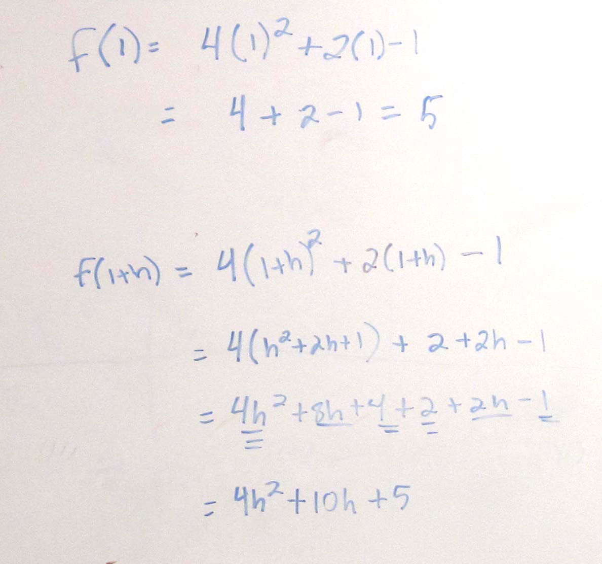
Example 1 Find the instantaneous rate of change of $latex \displaystyle f(x)=4{{x}^{2}}+2x-1$ at $latex \displaystyle x=1$.
Solution Start by calculating the two function values.
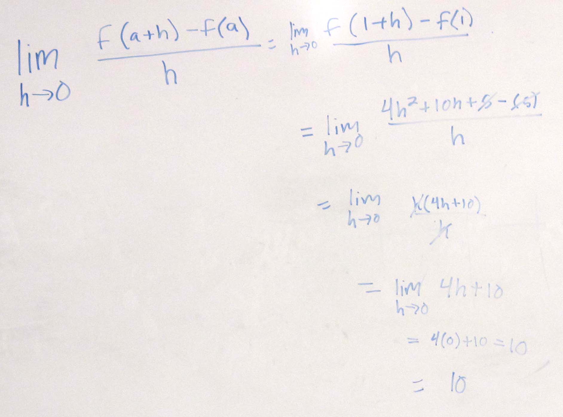
Once you have the function values, substitute them into the definition for instantaneous rate of change.
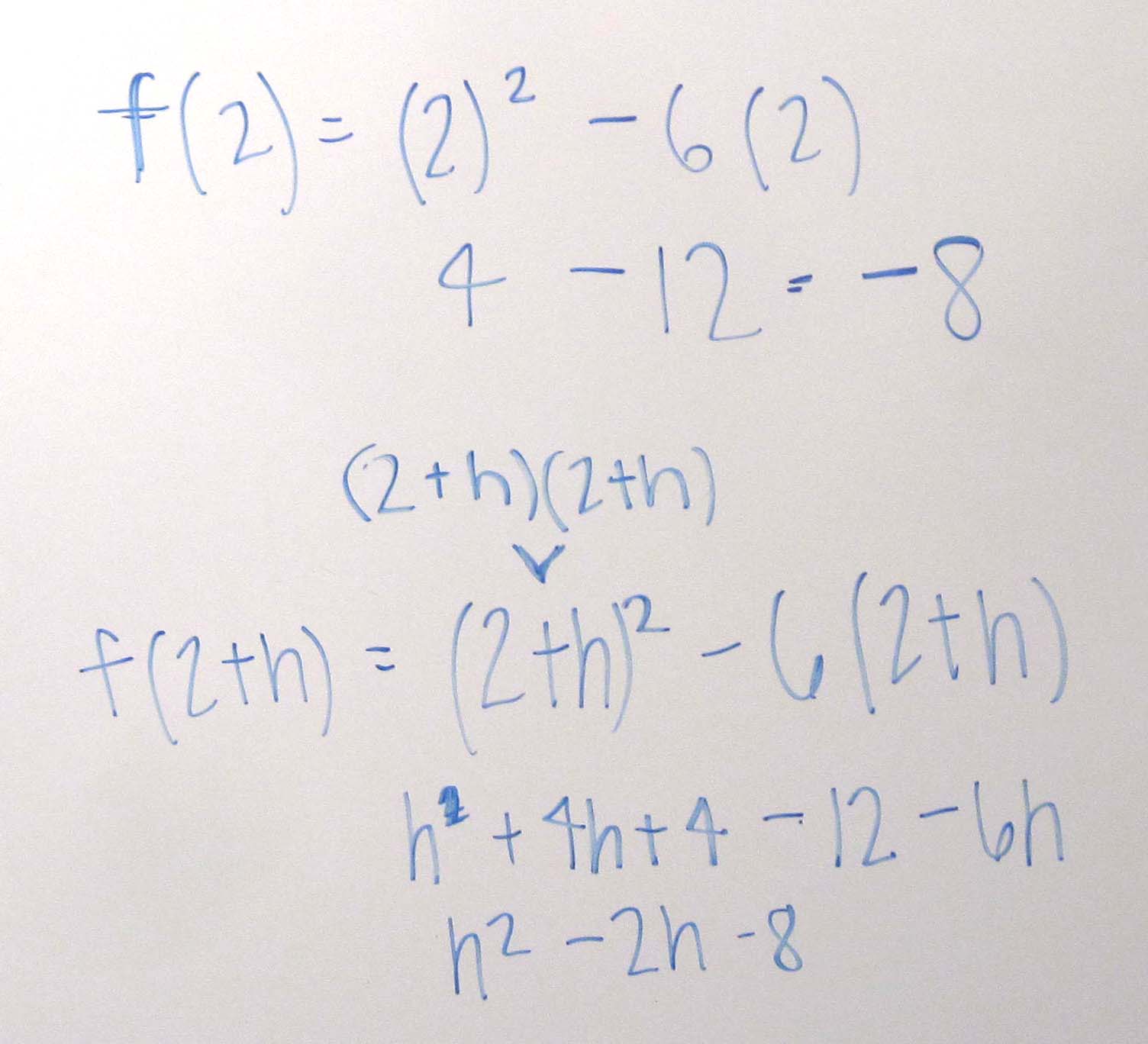
Example 2 Find the instantaneous rate of change of $latex \displaystyle f(x)={x}^{2}+6x$ at $latex \displaystyle x=2$.
Solution The function values are
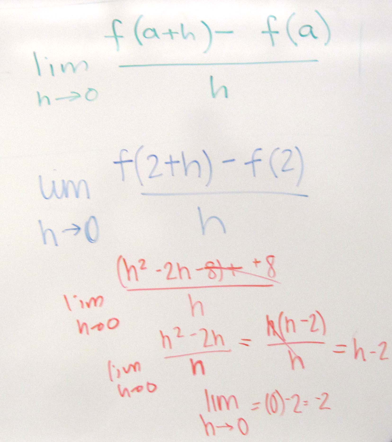
Now put these into the limit definition of instantaneous rate of change.
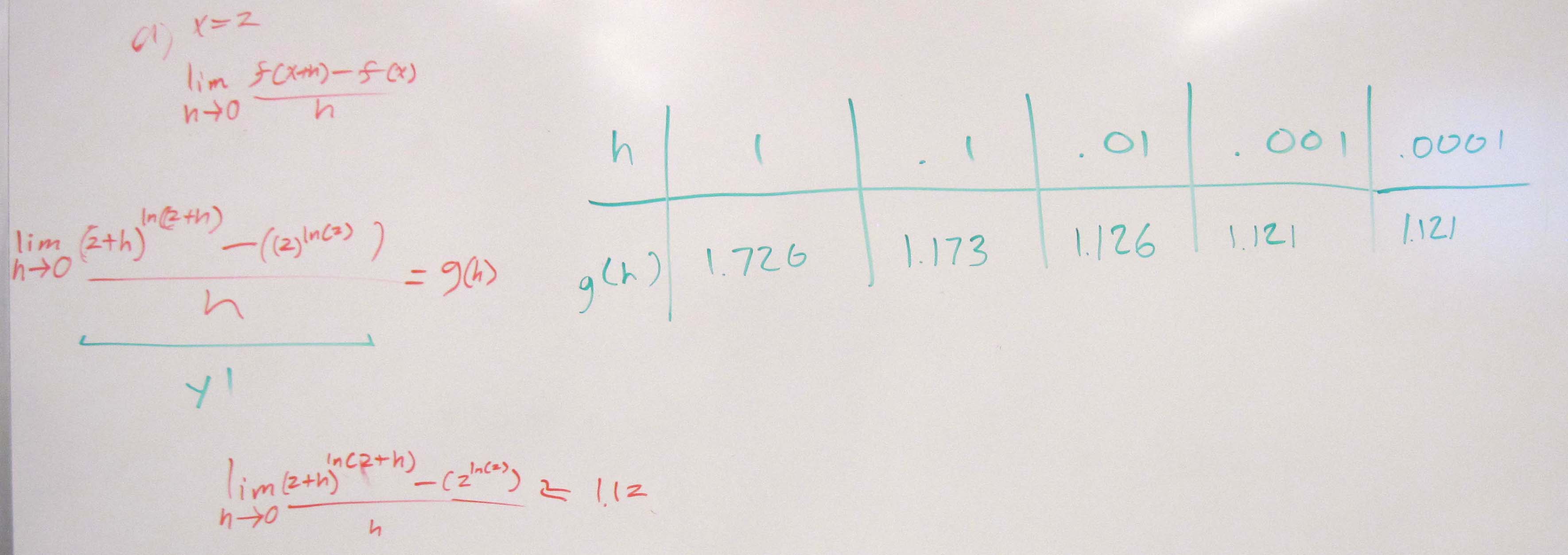
Problem 1 Estimate the instantaneous rate of change of f with respect to x at x = 2 if
$latex \displaystyle f(x)={{x}^{\ln (x)}}$
Solution In this problem, a = 2. We need to evaluate
$latex \displaystyle \begin{matrix}
\text{Instantaneous rate of change of }f\text{ } \\
\text{with respect to }x\text{ at }x=2 \\
\end{matrix}=\underset{h\,\,\to 0}{\mathop{\lim }}\,\frac{f(2+h)-f(2)}{h}$
Since the values in the table are shown to three decimal places, we can estimate the rate to two decimal places. In the last two columns, the difference quotient rounds to 1.12 so the rate is approximately 1.12.
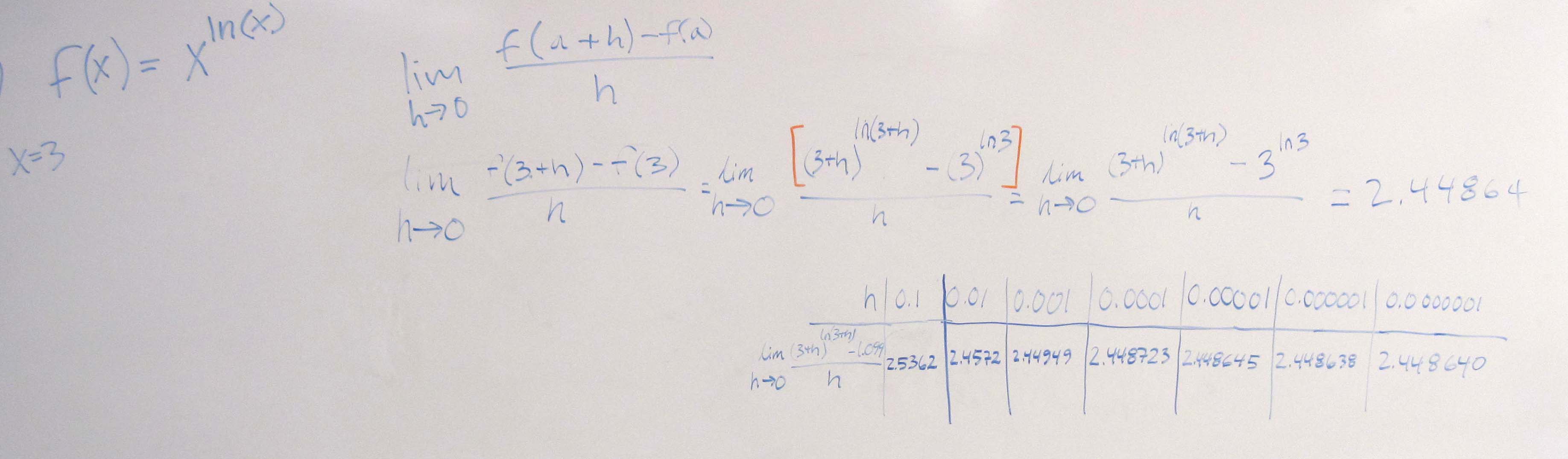
Problem 2 Estimate the instantaneous rate of change of f with respect to x at x = 3 if
$latex \displaystyle f(x)={{x}^{\ln (x)}}$
Solution In this problem, a = 3. We need to evaluate
$latex \displaystyle \begin{matrix}
\text{Instantaneous rate of change of }f\text{ } \\
\text{with respect to }x\text{ at }x=3 \\
\end{matrix}=\underset{h\,\,\to 0}{\mathop{\lim }}\,\frac{f(3+h)-f(3)}{h}$
The table shows most values to 6 decimal places. In the last two columns, the values both round to 2.44864.
There are several ways we can define elasticity E. Each indicates how the quantity demanded changes as the price is changed. In the examples below, we’ll utilize elasticity defined as