Category: Finite Mathematics Ebook

How do you find cost, revenue and profit functions with several variables?

In Example 3, we examined a cost function of several variables. This proved useful for modeling the total cost in a business that produces several different goods like milk. If the company receives revenue from several different products, we can utilize the fact that the revenue from each individual product by multiplying the price per unit times the number of units sold to get the revenue for that product. By summing the revenue for each of the products, we can form a model for the total revenue.

In the next example, we’ll continue working with the organic dairy from Example 3 to model the total revenue from selling three types of milk.

Example 4     Organic Dairy Revenue

The organic dairy in Example 3 charges $3.49 per gallon for whole milk, $4.19 per gallon for 2% milk, and $4.59 per gallon for 1% milk. If the variables Q₁, Q₂, and Q₃ represent the number of gallons of whole, 2% and 1% milk produced and sold respectively, find a linear function R(Q₁, Q₂, Q₃) to model the total revenue.

Solution We’ll find a linear function of the variables Q₁, Q₂, and Q₃. The coefficients in this function correspond to the increase in revenue from increasing the number of gallons of each type by 1 unit. These coefficients are simply the prices the dairy charges for one gallon of each type of milk. The linear function will have the form

R(Q₁, Q₂, Q₃) = p₁ Q₁ + p₂ Q₂ + p₃ Q₃

where p₁, p₂, and p₃ are the price per gallon for each type of milk.

Notice that there is no constant term in the sum since producing and selling no milk leads to no revenue. If we had included a positive constant, this would have been interpreted as revenue corresponding to (Q₁, Q₂, Q₃) = (0, 0, 0). With the prices in place, we get a linear model for total revenue in dollars,

R(Q₁, Q₂, Q₃) = 3.49Q₁ + 4.19Q₂ + 4.59Q₃

---

It is very common for cost and revenue functions to have many variables. Each variable corresponds to a unique product or service that a business provides to consumers. The coefficients of the cost function represent the variable costs per unit for each product or service and the constant represents the fixed costs of production. The coefficients of the revenue function represent the unit price for each product or service.

Example 5     Profit

The cost function for the organic dairy is

C(Q₁, Q₂, Q₃) = Q₁ + 1.1Q₂ + 1.25Q₃ + 10,000

and the revenue function is

R(Q₁, Q₂, Q₃) = 3.49Q₁ + 4.19Q₂ + 4.59Q₃

where Q₁ is the number of gallons of whole milk, Q₂ is the number of gallons of 2% milk, Q₃ is the number of gallons of 1% milk that the dairy produces and sells.

a. Find the profit function Profit(Q₁, Q₂, Q₃).

Solution Profit is the difference between revenue and costs,

b. Find the profit per unit for each type of milk.

Solution The coefficients on the profit function correspond to the change in profit when the corresponding variable is increased by 1 unit. Since the coefficient of Q₁ is 2.49, the profit increases by $2.49 when 1 more gallon of whole milk is produced and sold. This is the profit per gallon for whole milk. The same reasoning for the other types of milk leads to a profit per unit for 2% milk of $3.09 per gallon and $3.29 per gallon for 1% milk.

---

In real applications, the units are often modified to make the numbers more manageable. In Example 2, we examined the sales of a business in thousands of dollars given by S(A, E) = 105A + 1412E where A is the amount spent on advertising in thousands of dollars and E is the number of employees. If we were to find a value for this function like

S(10, 5) = 105(10) + 1412(5) = 8110

We would interpret this as indicating that advertising expenses of $10,000 and using 5 employees would lead to sales of $8,110,000. The variable A is scaled in thousands of dollars. Scaling a variable means that the actual amount is divided by an amount to obtain the value for the variable. In this case, dividing $10,000 by $1000 yields A = 10.

The dependent variable, sales, is also scaled in thousands of dollars. If we are given a value for this variable like 8110, we need to multiply by $1000 to get the actual amount. The value 8110 thousand dollars is the same as 8110($1000) or $8,110,000.

When independent variables are scaled, the cost and revenue functions change. In Example 3, we found the revenue function for an organic dairy that charges $3.49 per gallon for whole milk, $4.19 per gallon for 2% milk, and $4.59 per gallon for 1% milk. The function describing the revenue was

R(Q₁, Q₂, Q₃) = 3.49Q₁ + 4.19Q₂ + 4.59Q₃

where Q₁ is the number of gallons of whole milk, Q₂ is the number of gallons of 2% milk, and Q₃ is the number of gallons of 1% milk that the dairy produces and sells. Since an organic dairy might produce and sell thousands of gallons of each week, we could choose to scale the independent variables in thousands of gallons. Instead of inputting values like 1000 into a variable, we would input 1 instead. This introduces subtle changes into the revenue function since changes of 1 unit in the scaled variable results in a change of 1000 in gallons of milk. Let’s look at how this will change the revenue function.

Let R(Q₁, Q₂, Q₃) = p₁ Q₁ + p₂ Q₂ + p₃ Q₃ represent the revenue for the organic dairy where Q₁, Q₂, and Q₃ are the amounts of whole, 2%, and 1% milk in thousands of gallons produced and sold respectively. As we found in Example 3, the coefficients p₁, p₂, and p₃ are the unit prices of each type of milk. However, when the variables are scaled the meaning of one unit changes. Now the unit price corresponds to the price of 1 thousand gallons of milk. A price of $3.49 per gallon is equivalent to $3490 per 1 thousand gallons of milk. If we change each unit price to account for the scaling, we get

R(Q₁, Q₂, Q₃) = 3490Q₁ + 4190Q₂ + 4590Q₃

The value

R(0, 2, 0) = 3490(0) + 4190(2) + 4590(0) = 8380

represents the revenue from producing and selling 2000 gallons of 2% milk.

If we were to calculate the same revenue from the function in Example 3, we would get

R(0, 2000, 0) = 3.49(0) + 4.19(2000) + 4.59(0) = 8380

The key part of each calculation is middle term,

In each case, the units in red reduce to 1 leading to a function value of 8380 dollars. By examining the units carefully in each term, we can deduce the units on the revenue. The units on each term must be the same for the terms to add together properly.

Another possibility is to scale the variables in thousands of gallons but use the unit prices in dollars per gallon. In this case the middle term would be

In this case, the numbers multiply to 8.38 and the units are thousands of dollars.

To define the function with the revenue in thousands of dollars we would write the function as

R(Q₁, Q₂, Q₃) = 3.49Q₁ + 4.19Q₂ + 4.59Q₃

with each of the variables scaled in thousands of gallons. Now the revenue from 2000 gallons of 2% milk is calculated as

R(0, 2, 0) = 3.49(0) + 4.19(2) + 4.59(0) = 8.38

and the revenue is 8.38 thousand dollars or $8380.

Each of these models may be used to calculate the revenue for the organic dairy. However, the units you choose for the independent and dependent variables in the revenue and cost functions should match. If not, you might find yourself subtracting cost in dollars from revenue in thousands of dollars. This would lead to a value for profit that makes no sense.

What do the coefficients of the variables tell us?

For a linear function of one independent variable, the coefficient on the variable is the slope or rate of change. We can generalize this idea to linear functions of several variables. Let’s consider the function g (x₁, x₂) = 2x₁ – 3x₂. As we saw in Example 1, we can substitute values for the variables to obtain a value for the function. For instance, if we want to substitute 10 for x₁ and 2 for x₂ we get

g (10, 2) = 2(10) – 3(2) = 14

Now compare this value to the value obtained when we increase the value for x₁ by 1 unit,

g (11, 2) = 2(11) – 3(2) = 16

The difference between these values is g (11, 2) – g (10, 2) = 16 – 14 = 2. Since the coefficient on  is a 2, increasing the value for  increases the value from g by 2 units. The coefficient on  tells us the amount the function will change when  increases by 1 unit.

In general, this applies for any value of x₁. If we fix x₂ at some value and find the difference between the function at x₁ and at x₁ + 1 we get

We can also apply this reasoning to the coefficient of x₂. If we fix x₁ at some value and find the difference between the function at x₂ and x₂ + 1 we get

The coefficient on x₂, -3, indicates the amount the function will change when grows by 1 unit.

This leads to the following generalization.

Example 2     Interpret Coefficients

The function S(A, E) = 105A + 1412E describes the monthly sales, in thousands of dollars, at a large dairy distributor with E employees and A thousand dollars of monthly advertising costs.

a. What does the coefficient of E tell you about the monthly sales?

Solution The coefficient of E, 1412, relates the change in sales to the variable E when it is increased by 1 unit. An increase of 1 unit in E means an increase of 1 employee. This leads to an increase in sales of 1412 thousand dollars or $1,412,000.

b. What does the coefficient of A tell you about monthly sales?

Solution The coefficient of A, 105, relates the change in sales to the variable A when it increases by 1 unit. An increase of 1 unit in A means an increase of 1 thousand dollars in advertising. This leads to an increase in sales of 105 thousand dollars or $105,000.

---

We can now interpret what coefficients a₁ through a_n mean, but what about the constant a₀? The constant a₀is similar to the vertical intercept b for a linear function of one independent variable . In that case, b is the value of the function when the variable is set equal to zero, f (0) = m(0) + b = b. For a linear function of n independent variables, the corresponding process is to set all independent variables equal to zero. If f (x₁, x₂,…, x_n) = a₀ + a₁ x₁ + a₂ x₂ + …+ a_n x_n, we can set each variable equal to zero to obtain

f (0, 0,…, 0) = a₀ + a₁ (0) + a₂ (0)+ …+ a_n (0) = a₀

The only term that remains is the term containing the constant a₀.

Example 3     Fixed Costs for an Organic Dairy

The daily cost function (in dollars) for an organic dairy is given by the linear function C(Q₁, Q₂, Q₃) = Q₁ + 1.1Q₂ +1.25Q₃ + 10,000 where is Q₁ the number of gallons of whole milk produced, Q₂ is the number of gallons of 2% milk produced, and Q₃ is the number of gallons of 1% milk produced.

a. Find the fixed costs for the organic dairy based on this function.

Solution The fixed costs are costs incurred when nothing is produced. We can find this cost by finding C(0, 0, 0) or by noting that the constant gives the function’s value when all variables are zero. Either way, the fixed costs are $10,000.

b. How much does each additional gallon of 2% milk cost to produce?

Solution The coefficient of Q₂ gives the change in the cost when Q₂ is increased by 1 unit. In this case, the coefficient is 1.25 which tells us that another gallon of 2% milk will cost an additional $1.25.

---

We can calculate the amount it would cost to change production in Example 3 by any amount by adding the amount to the appropriate independent variable and utilizing the cost function. If we want to find the additional cost incurred from increasing the production of 1% milk by 1000 gallons, calculate

The extra 1000 gallons cost $1250. This number is independent of the initial production level. If we start with no 1% milk and increase production to 1000 gallons or increase production of 1% milk from 10,000 gallons to 11,000 gallons, the additional cost will be $1250. For linear functions like this one, the increase is always independent of the production level. Another way of thinking about this is that the variable costs for 1% milk are $1.25 per gallon. This is precisely the coefficient on the variable representing 1% milk, Q₃.

What is a linear function of several independent variables?

In section 1.1, we introduced a linear function of one variable, y = mx + b. There was nothing special about the names of the variables, x and y, or the names of the constants, m and b. Another possible form for a linear function of x and y is y = a₀ + a₁ x. In this format, a₀ is the vertical intercept and a₁ is the slope.

When several independent variables are introduced, it is prudent to use names for the variables that make sense. If one variable is named x, we can extend this to n variables using subscripts. Subscripts are numbers that appear to the right of the variable and slightly lowered. The subscript is a part of the variable’s name and is useful to show generically that there are many variables. For instance, if we wanted to define a function with three independent variables that describe the quantities of three different products, we might use Q₁, Q₂, and Q₃.

In general, let x₁, x₂, … , x_n be the names of n independent variables.

Function notation applies to functions of several independent variables as well as functions of one independent variable. Recall that a linear function of one variable x named f  would be written as f (x) = a₀ + a₁ x. The independent variable for the function is placed in parentheses after the name to distinguish the variables from the constants. For a linear function of n independent variables, the n independent variables are placed in the parentheses after the name to give

f (x₁, x₂, … , x_n) = a₀ + a₁ x₁ + a₂ x₂ + ··· + a_n x_n

Example 1      Find Function Values

If f (x₁, x₂, x3) = 10 – 2x₁ + x₂+ 3x₃, find the value of f (6, -1, 2).

Solution  Substitute x₁ = 6, x₂ = -1, and x₃ = 2 into the function to yield

f (6, -1, 2) = 10 – 2(6) + (-1)+ 3(2) = 3

 

How good is the linear model?

The linear model is not complete without an indication of how good the fit is to the data. We can examine the scatter plot with the model and data and get a qualitative idea of the fit, but this can be deceiving.

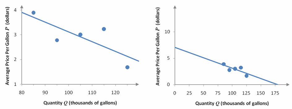
Figure 8 – Two scatter plots of the data in Table 1. The model of each scatter plot is P = -0.0395Q + 7.0675, but the horizontal and vertical scales are different.

Which linear model in Figure 8 appears to be a better fit? On the surface, you would probably say that the model on the right is a better fit. But in fact, both scatter plots depicts the exact same model with different scales. The vertical scale for the scatter plot on the right is larger and makes any gaps between the model and the data seem small. This makes the points appear to be closer to the line. In fact, the vertical distance between each data point and the line are exactly the same and there is no difference in the fit.

To remedy this and other difficulties in determining goodness of fit, two indicators are used. The correlation coefficient and coefficient of determination are commonly used to compare the fit of regression models.

A positive correlation coefficient indicates that the data is positively correlated. For linear models with a positive correlation coefficient, the slope of the model will be positive. A negative correlation coefficient indicates that the data is negatively correlated. For linear models with a negative correlation coefficient, the slope of the model will be negative.

Figure 9 – Three different sets of data and the corresponding linear models. The worst fit is in graph a with an absolute value of the correlation coefficient closest to 0. The best fit is graph c with an absolute value of the correlation coefficient closest to 1. Each model is decreasing so the correlation coefficient is negative.

As |r| gets closer to 1, the data points get closer to the linear model.

Another measure of fit is the coefficient of determination, r². For a linear model, the coefficient of determination is the square of the correlation coefficient . Since is a number from -1 to 1, r² is a number from 0 to 1. The closer the coefficient of determination is to 1, the more linearly related the data are. If the coefficient of determination is close to 0, the data are not linearly related.

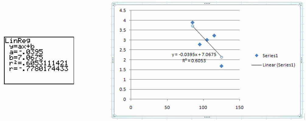
Figure 10 – A graphing calculator or Excel can be used to calculate the correlation coefficient or coefficient of determination. A graphing calculator (left) returns both values. Excel (right) can return the coefficient of determination (it is written as R² instead of r²).

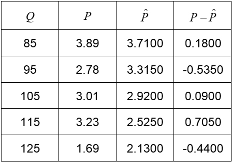
Another measure of how close the data lie with respect to the linear model is the percent error. The percent error at any value of the independent variable is found by dividing the error, , by the data value P. We can find the percent error by calculating

at each data value where P is the price data and  is the model’s estimate of the price. At Q = 115, the percent error is

or approximately 21.8%. This means that as a proportion of the price, the price at Q = 115 is 21.8% above the model’s estimate of the price.

Example 3      Find the Largest Percent Error

For the model P = -0.0395Q + 7.0675 and the data in Table 3,

Find the quantity that yields the largest percent error.

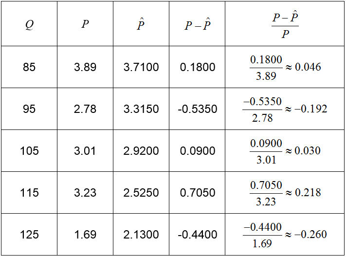
Solution  Add a column to the table and calculate the percent error at each quantity.

The largest percent error is 26% and occurs at Q = 125. This price is 26% below the linear model.

How do you use linear regression functions?

Once you have found a linear model using linear regression, you can use it to analyze problems. These problems may involve questions about the slope or the variables.

Example 1      Use a Linear Model

The least squares linear model for the data in Table 1 is P = -0.0395Q + 7.0675.

a.  Use this model to determine the average price when 100 thousand gallons of milk are sold.

Solution  This equation relates Q, the quantity of milk sold in thousands of gallons, to the average price P. Since we are given a value of substitute this into the model:

P = -0.0395(100) + 7.0675 ≈ 3.12

At a price of $3.12, 100 thousand gallons of milk are demanded per week.

b.  Use this model to determine the amount of milk sold per week when the average price per gallon is $2.90.

Solution  In this part, a price of P = 2.90 is specified. We can substitute this value into the model and solve for Q to get the quantity.

This fraction is approximately 105.506 thousand gallons of milk or about 105,506 gallons of milk per week.

---

Example 2      Interpret the Slope of the Model

The least squares linear model for the data in Table 1 is P = -0.0395Q + 7.0675. Use this model to determine the rate at which the prices are changing with respect to quantity.

Solution The rate at which the variables change with respect to each other is the slope of the model.

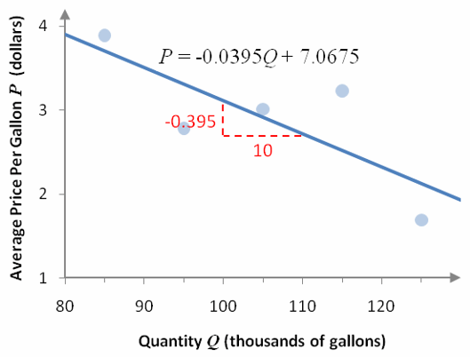
Figure 7 – A graph of the model with the slope labeled as a ratio.

The slope, -0.0395, is the coefficient of the independent variable Q. However, giving the number as the rate is not complete. A rate should include units. This allows you to understand what the rate means.

In Figure 7, the slope of the model is labeled so that the ratio of the vertical change to the horizontal change is

This tells us that for every 10,000 gallon increase in demand, the price per gallon drops .395 dollars or 39.5 cents.

We could also write the ratio as

In this case, we would interpret this as a decrease of 10,000 gallons in demand leads to an increase in price of .395 dollars or 39.5 cents.

In general, rates are interpreted in 1 unit increments of the independent variable. Writing the ratio as

means that for every 1 thousand gallon increase in demand, the price drops by 0.0395 dollars or 3.95 cents. We can state this easily by saying that the rate is -0.0395 dollars per thousand gallons. The units include the term “per” meaning that the units are a ratio of dollars to thousands of gallons.