Section 1.3 Question 1

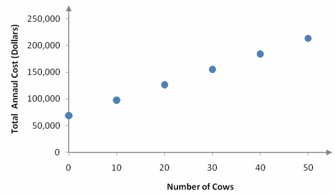
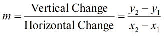
Which linear model is best?

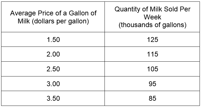
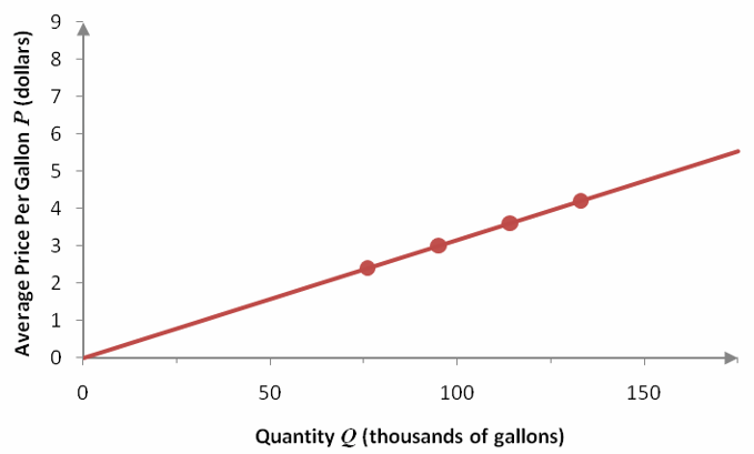
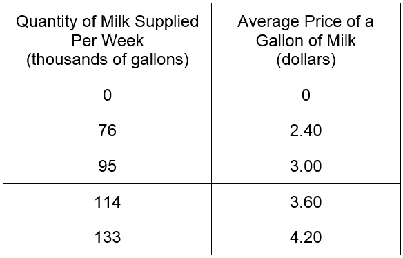
In real life, data are not so perfect. A more common situation might be the data in Table 1.
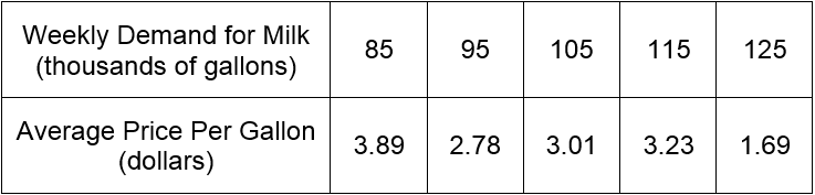
1_3_1_1

Table 1

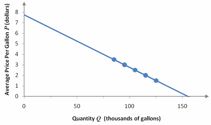
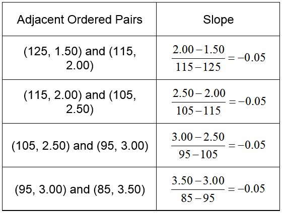
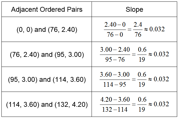
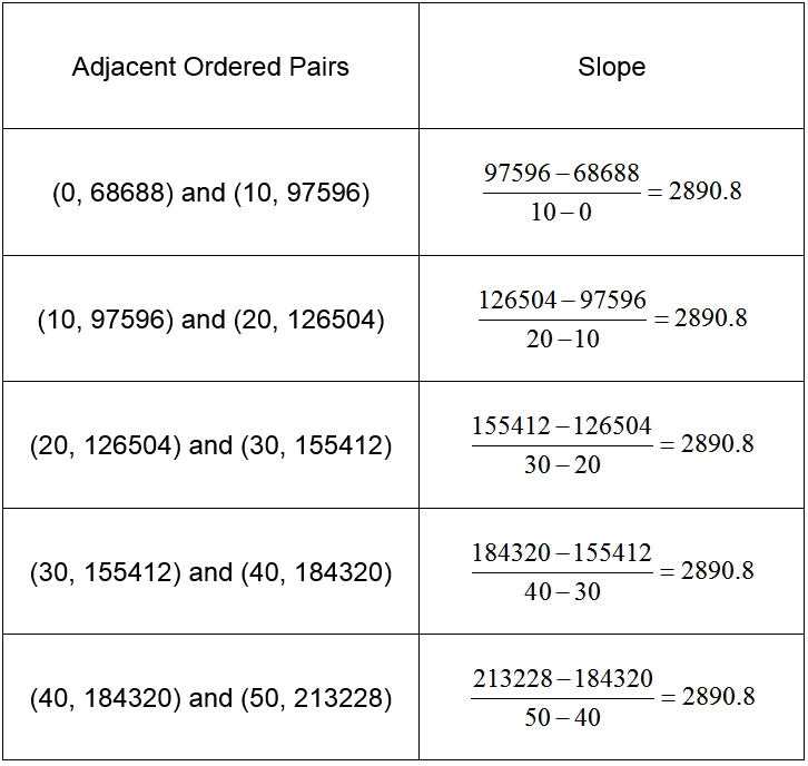
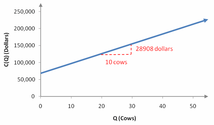
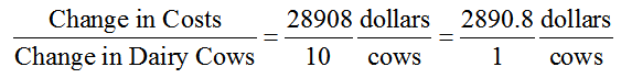
If we were to calculate the slope between adjacent points, we would find that the slope is not constant. This is easy to see if we graph the ordered pairs from the table in a scatter plot.

1_3_1_2

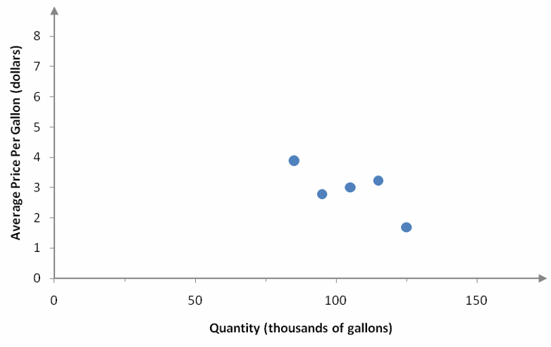
Figure 2 – A scatter plot of the data in Table 1.

The slope between adjacent ordered pairs is not constant.

Although we cannot find a linear function that passes though all of the points, we can find a linear function that passes close to the points. This function is said to model the data. A mathematical model is a representation of a real world system. In this case, the model is a representation of the relationship between the average price of a gallon of milk and the quantity of milk sold per week.

1_3_1_3

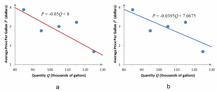
Figure 3 – Two different linear functions that model the relationship between the average price of a gallon of milk and the number of gallons sold at that price.

The linear functions in Figure 3 both pass close to the points, but which function passes “closest” to the points?

Closeness is measured vertically from the data point to the line. For instance, let’s draw a vertical dashed line from each point to the linear function in Figure 3a.

1_3_1_4

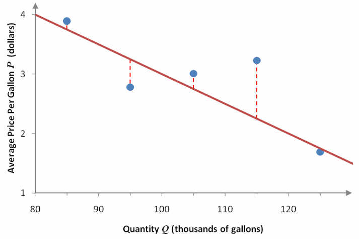
Figure 4 – The dashed red lines represent the vertical distances between the data values and the linear function.

The vertical distance between any data value and the line can be computed by subtracting the corresponding prices. To find the largest vertical distance at Q = 115, we need to find the average price from the data and from the linear model:

Price at Q = 115 from data:   P = 3.23

Price at Q = 115 from linear function:      1_3_1_5

The symbol 1_3_1_6 indicates that the price has been estimated from the model whereas P indicates a data price. The difference between the data price and the linear model price is called the error or residual. For this price, the error is

1_3_1_7

Since the error is positive, we know that the data price is higher than the model’s price. If the error is negative, the model’s price is higher than the data price. This is the case at Q = 95:

Price at Q = 95 from data:    P = 2.78

Price at Q = 95 from linear function:          1_3_1_8

1_3_1_9

We can carry this process at each of the quantities in Table 1 and label it on a scatter plot.

1_3_1_10

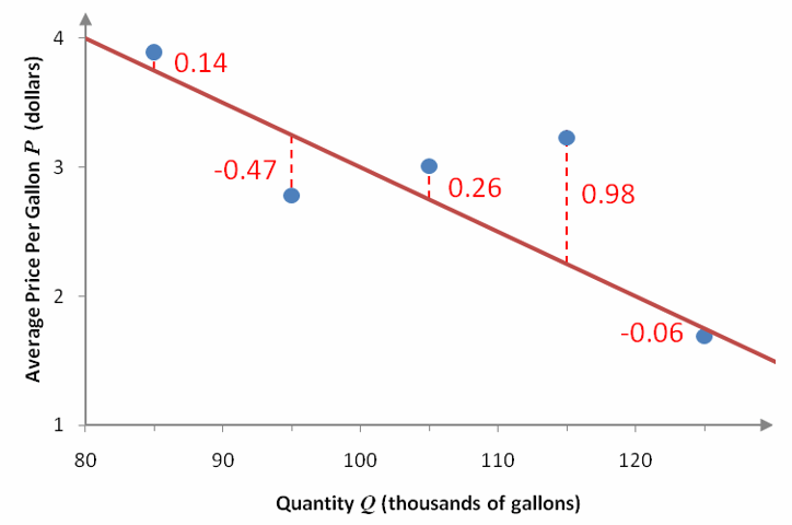
Figure 5 – A scatter plot of the data and the linear model. The dashed red line and red numbers indicate the error between the data and the model.

If we want a linear function to go as close to the ordered pairs as possible, we need to collectively make these errors as small as possible. This is done by summing the errors at each quantity.  If the sum of the errors is zero, the linear function might go through each point.

1_3_1_11

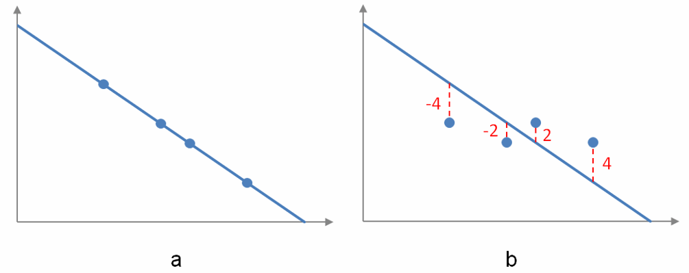
Figure 6 – In a, each data point coincides with the linear model so the sum of the errors is zero. In b, the sum of the errors is also zero, but the data points do not lie on the graph of the linear model.

But we can’t simply sum the errors as is since some of the errors are positive and some are negative. By adding the errors together we might have some cancellation and be deceived into thinking that a linear model coincides with the data when it does not. This situation is illustrated in Figure 6. In graph a of Figure 6, each ordered pair of the data lies on the linear model so there is no error between the model and the data. The sum of the errors is zero. In this case, the linear model fits the data perfectly.

But simply adding the errors is inadequate. In graph b of Figure 6, the sum of the errors is also zero. However the model does not fit the data perfectly. Some ordered pairs are above the linear model and others are below the linear model. For each positive error, there is a negative error that cancels it. Even though the sum is zero, the linear model is not a very good fit for the data.

A better criterion for determining the fit is needed. Instead of simply summing the errors, sum the square of the errors. This eliminates the potential cancellation of the positive and negative errors.
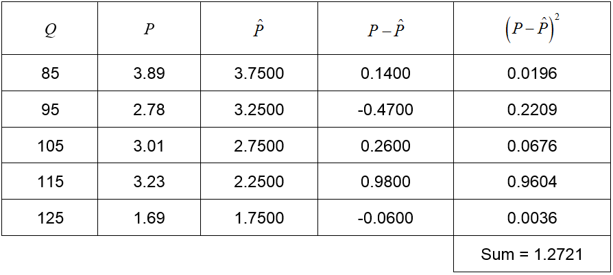
1_3_1_12

Table 2

In Table 2, the first three columns describe the quantity Q, the price P and the estimate of the price  based on the linear model. The fourth column describes the error in the estimate and the last column corresponds to the squared error. For this model, the sum of the squared errors is 1.2721.

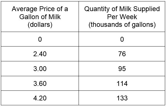
A model that has a lower sum of squared error would be considered a better model. Let’s look at the model in Figure 3b, P = -0.0395Q + 7.0675.
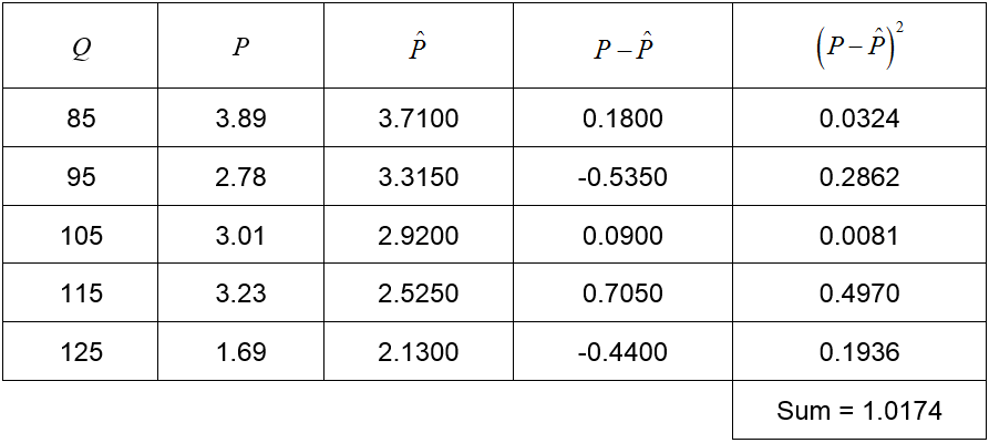
1_3_1_13

Table 3

This model, rounded to four decimal places, is better since the sum of the squared errors is lower.

The model P = -0.0395Q + 7.0675  in Table 3 is the very best model for the data. This means that it has the lowest sum of squared errors. If we were to vary the slope and intercept in the model, no other combination would lead to a sum lower than 1.0174.

The process of calculating the linear model with the smallest sum of squared errors is called linear regression. The model obtained through linear regression goes by several different names. Best linear model, least squares linear model and best line are all terms that can be used when referring to the model. The model is typically obtained using technology like a graphing calculator or Excel. The formulas required for calculating the slope and intercept of the best linear model without technology uses calculus and are beyond the scope of this text.

Section 1.2 Question 5

What are demand and supply?

An important application of linear functions is the connection between the price of a good or service and the quantity of a good or service. If we are interested in the relationship between the price and the quantity demanded by consumers at that price, this connection is described by the demand function. The relationship between price of a good or service and the quantity supplied by manufacturers at that price is described by the supply function. These functions describe how consumers and suppliers behave as price is changed.

The consumer’s behavior is given by a table called a demand schedule. This table reflects the relationship between the price of some good or service and the quantity of this good or service demanded at this price. The table below is a typical demand schedule in some market.

1_2_5_1

In the first column of the demand schedule are prices of some good. In the other column is the corresponding numbers of that good sold to consumers. From this demand schedule for dairies in a competitive market, we can see that as the price per gallon for milk increases the quantity of milk sold per week decreases. The law of demand states that if everything else is held constant, as the price of the good increases, the quantity demanded drops. This pattern is visible in the demand curve shown below.

The demand function is traditionally graphed with the quantity as the independent variable and the price as the dependent variable. Because of this, quantity is graphed on the horizontal axis and price is graphed on the vertical axis. This means that the information indicating that 125,000 gallons of milk is sold per week at a price of $1.50 per gallon corresponds to the ordered pair (125, 1.50). The demand function takes an input of quantity and outputs price,

P = D(Q)

Demand curves can have many shapes, but the simplest curve is a demand curve follows a straight line. In the case of the demand function for dairies in a market shown here, we’ll find a linear demand function of the form

D(Q) = mQ + b

This is the same form defined earlier, (x) = mx + b, with the variable changed to Q from x and the name changed to D from f.

1_2_5_2

Figure 11 – The demand D(Q) for milk.

Example 6      Find the Demand Function for Milk

Find the equation of the demand curve graphed in Figure 11.

Solution  The graph above gives us a hint that the demand function is a linear function. To make sure the ordered pairs all lie along a straight line, we need to find the slope between adjacent ordered pairs.

1_2_5_3

Table 6

Since the slope between any pair of adjacent points is -0.05, all of the points lie along a line with slope -0.05.

Insert the slope into the form for a linear demand function to yield

D(Q) = -0.05Q + b

All that remains is to find the vertical intercept b in the function. None of the points are the vertical intercept. To find b, substitute any of the points into the function. Let’s try the ordered pair (125, 1.50):

D(125) = -0.05 (125) + b = 1.50

To find the value of b, simplify the equation to give

-6.25 + b = 1.50

Adding 6.25 to both sides leads to b equal to 7.75. The function for demand is

D(Q) = -0.05Q + 7.75


The supply function also relates the price of a good or service to a quantity of the good or service. Unlike the demand function which describes the consumer’s willingness and ability to buy a good or service, the supply function describes the willingness and ability of a business to supply a good or service at a given price. If all other factors are held constant, as the price rises the quantity supplied will also increase. A higher price leads to more profit for a business encouraging higher production.

A supply schedule is a table that shows the relationship between the price of a good or service and the quantity supplied by a firm.

1_2_5_4


Table 7

In this supply schedule, an increase in the average price of a gallon of milk corresponds to an increase in the quantity of milk supplied by dairies. A graph of the data shows a straight line with a positive slope.

1_2_5_5

Figure 12 – Data from the supply schedule and the corresponding supply curve.

Keep in mind that while this is a “typical” supply schedule, supply functions may have many different shapes. A supply function may be curved concave down or up. It may even change its concavity.

1_2_5_6

Figure 13 – Three examples of supply functions. In a, the supply curve is concave down. In b, the supply curve is concave up. In c, the supply curve changes from concave down to concave up.

A linear function often models the data adequately and simplifies later calculations. A linear supply function has the form

S(Q) = mQ + b

where m is the slope of the line and b is the vertical intercept.

Example 7      Find the Supply Function for Milk

Find the linear supply function S(Q), where Q is the quantity of milk supplied, passing through the ordered pairs in Table 7.

Solution  Since the function will be a function of Q, interchange the columns of the table. This change is necessary since the independent variable is typically listed in the first column.

1_2_5_7

Let’s check the slope between adjacent points.

1_2_5_8

Table 8

The fractions 2.4/76 and 0.6/19 simplify to 3/95. Since all of the slopes are the same at about 0.032, we know the points lie along a straight line.

Unlike the demand function, we know that the vertical intercept is (0, 0) so the equation of the line is

1_2_5_9

Notice that the fraction has been used for the slope. If the rounded decimal had been used instead of the exact fraction, the line would go very close to the data in the supply schedule, but not through exactly. Decimals are acceptable when they are exact decimals and not rounded or where approximations are acceptable.


Example 8      Find the Surplus at a Fixed Price

At a price of $3.36 per gallon, dairies will be willing to supply more milk than consumers are willing to buy. Find the surplus amount of milk at this higher price.

Solution  To find the amount of the surplus, we must find the difference between the quantity supplied and the quantity demanded. These quantities are found by setting the outputs of the supply and demand functions equal to $3.36.

To find the quantity supplied, set S(Q) equal to 3.36 and solve for the quantity Q :

1_2_5_10

At a price of $3.36 per gallon, the dairies would be willing to supply 106.4 thousand gallons or 106,400 gallons of milk per week.

To find the quantity demanded by consumers, set D(Q) equal to 3.36 and solve for Q:

1_2_5_11

The demand at a price level of $3.36 per gallon is 87,800 gallons of milk per week.

The surplus of milk is the difference between the two quantities or

Surplus = 106,400 – 87,800 = 18,600 gallons per week

Section 1.2 Question 4

How do you find cost and revenue functions?

All businesses produce some kind of product. That product may be something that you can hold in your hand like an MP3 player or it may be a service like cleaning an office. The outputs from the business take the form of goods and services. To produce these outputs, the business requires inputs such as workers, machines and supplies. A business takes the inputs and converts them to outputs.

The process of converting inputs to outputs requires technology. This is more than our everyday meaning where we think of technology as a cool new product or technique. In economics, technology is any process a business uses to convert inputs into outputs. It depends on many factors. For instance, in a dairy the factors might include the capacity of the milking machinery, the skill of the laborers who operate the machinery and the quality of the feed the cows are fed.

Technological change may occur if the businesses inputs and outputs change. This can occur in two basic ways. First, there may be a change in the outputs for the same number of inputs. If greater output occurs for the same level of inputs, positive technological change has occurred.  If lower output occurs for the same level of input, negative technological change has taken place. For instance, if a dairy produces more milk with the same number of cows, positive technological change has taken place.

Technological change can also take place if the outputs are held constant and the inputs change. Positive technological change occurs if the same output occurs, but from a lower level of inputs. On the other hand, negative technological change occurs if the same outputs occur for an increased level of inputs. If a dairy produces the same amount of milk from fewer cows, positive change has taken place. If it takes more cows to produce the same level of milk, negative change has taken case.

Businesses are interested in knowing the relationship between the inputs and outputs with respect to the costs they incur to produce the outputs. Since there can be many different inputs that affect their costs, at least one of the businesses input are held constant. This period of time is called the short run. The period of time for which any of the businesses inputs can vary or it can change its technology or capacity is called the long run.

Let’s consider several inputs for a dairy that could lead to the output of milk. A dairy could change the number of cows producing milk, the number of breeding cows, the number of laborers, the capacity of the milking machines, the type of feed or the number of acres used to graze the cows on. The long run is the period of time over which the dairy can vary all of these inputs. The short run is the period of time over which at least one of the inputs is fixed. If the number of cows producing milk is varied over a year, but all other inputs are fixed, the short run is a year. Depending on what is fixed and what is left to vary influences the short run.

To examine the total cost of producing outputs, it is often easiest to look at the short run and to fix as many of the inputs as possible. If only one variable changes, the total cost function will contain only one variable. A total cost function with two variables means that two inputs are varied and so on.

Costs typically fall into two categories, variable costs and fixed costs. To determine which category a cost falls, we need to examine how the cost changes as the outputs change. If a cost varies as the output changes, the cost is a variable cost. A cost that does not change as the output changes is a fixed cost. For a dairy, the labor costs, veterinary costs, feed costs, and utility costs change as the output level of milk changes. To produce more milk, more people need to feed and milk the cows. More milk also means that it will cost more to maintain the health of the herd as well as to operate the milking machines. Costs like real estate taxes, interest on short term loans, and depreciation on equipment are fixed as milk production changes and would be considered fixed costs. All costs are either variable or fixed.

The total cost of operating the business is the sum of the variable costs and the fixed costs,

Total Cost = Fixed Cost + Variable Cost

For a cost function in which all inputs are fixed except one, a single variable is used and the cost function is called C(Q) or Cost(Q). The variable Q is the input that is varied and needs to be defined so that the function makes sense.

Example 4     Dairy Costs

Use Table 2 to find a function that describes the total annual costs C(Q) of running a dairy as a function of the number of cows Q producing milk. By saying “annual”, we are assuming that the short run is a period of one year. Since the function C(Q) has only one input Q, all others are being held constant in the short run.

The table below describes the fixed, variable and total costs as the number of dairy cows is increased.

1_2_4_1

Table 2

Solution Notice that in each row of Table 2, the total cost is the sum fixed cost and the variable cost.

Let’s get a feel for C(Q) by graphing the pertinent columns of this table in a scatter plot. The variable Q represents the number of dairy cows so this will be the input or independent variable on the scatter plot. The dependent variable represents the total cost. This means that we’ll graph the first and fourth columns of the table as ordered pairs,

1_2_4_2

The scatter plot of the ordered pairs is shown below.

1_2_4_3

Figure 7 – Scatter plot of data in Table 2

The ordered pairs appear to follow a straight line. To check, let’s calculate the slope between adjacent points on the graph.

1_2_4_4

Adjacent sets of points have the same slope, 2890.8, so all points lie along a line.

The slope of the line is 2890.8 and the vertical intercept is 68688. Since the graph corresponds to a linear function, we can write the total cost function as

C(Q) = 2890.8Q + 68688

where Q is the number of dairy cows.  The term 68688 is fixed as Q changes and corresponds to the fixed costs.

1_2_4_5

Figure 8 – The linear function corresponding to the data in Figure 7.

The slope indicates the rate at which costs are changing. In this case, we can think of the slope as

1_2_4_6

This tells us that increasing the number of cows by one increases the total cost by 2890.8 dollars. Thus the variable term 2890.8Q corresponds to the variable cost since the term changes as Q changes.

The slope is also called the marginal cost since it describes how the costs change when the input changes by 1 unit. In general, the term marginal describes how one quantity changes when the input changes by 1 unit.


As discussed before, businesses convert inputs to outputs. This process costs businesses money which is described by the total cost function C(Q). To compensate for these costs, businesses receive money for selling goods or services. The amount received depends on the inputs to the businesses and is called revenue. The revenue function is denoted by the name R or the name Revenue and is a function of the company’s inputs. Typically revenue is described in the short term where at least one of the inputs is fixed. If all but one of the inputs are fixed, the revenue can be denoted by a function of one variable R(Q) or Revenue(Q).

Example 5      Dairy Revenue

A dairy can increase its milk production and thus its revenue in several ways. By changing the feed or administering certain hormones, the amount of milk produced can be increased and lead to higher total revenue. Revenue can also be changed by increasing or decreasing the number of dairy cows. More cows can produce more milk thus leading to higher revenue. We are interested in varying the number of cows Q and seeing how the total annual revenue R(Q) changes. All other inputs to the business will be held constant in the short run.

The table below describes the level of total annual revenue for various numbers of dairy cows.

1_2_4_7

Table 4

Find the revenue function R(Q).

Solution This is a function of the number of dairy cows. On a graph, we know that the number of dairy cows will be graphed horizontally and the total annual cost will be graphed vertically.

1_2_4_8

Figure 9 – Scatter plot of data in Table 4.

Like the total annual cost, the total annual revenue appears to follow a straight line. Let’s calculate the slope between adjacent points.

1_2_4_9

Table 5

The slope between any pair of points on the line is 3547. This indicates that the ordered pairs all lie along a line that has a slope of 3547. Since the vertical intercept of this line is the point (0,0), we can use the slope-intercept form of a line to write

R(Q) = 3547Q

The graph of this function mirrors the trend of the data in the scatter plot above.

1_2_4_10

Figure 10 – The linear function corresponding to the data in Figure 9.

We can think of the slope of the revenue function as a ratio,

1_2_4_11

An increase in the number of dairy cows by 10 leads to an increase in revenue of $35,470. This means that each additional dairy cow adds $3547 to the revenue. The amount of revenue added when the input increases by one unit is called the marginal revenue.

Section 1.2 Question 3

How do you find a linear function through two points?

The examples above demonstrate how to create points with a given slope between them. This is useful if we are given the function to begin with. However, we may also be given at least two points on the graph of the function and want to find the function’s formula. In this case we need to find the slope of the line passing through the points.

Suppose you are given two points (x1, y1),  and (x2, y2), on a line. The slope of the line is found by calculating

1_2_3_1

When you use this formula be careful to subtract the y values in the numerator (the vertical change) and the x values in the denominator (the horizontal change). Also that you subtract in the proper order.

Example 2      Find the Slope Between Two Points

For each part, find the slope of the line passing through the two points.

a. (3, 1) and (5, 8)

Solution  Let  (x1, y1) = (3, 1) and (x2, y2) = (5, 8) . Substitute these ordered pairs into the slope formula to yield

1_2_3_2

b. (-3, 2) and (4, -1)

Solution  Let  (x1, y1) = (-3, 2) and (x2, y2) = (4, -1). Substitute these ordered pairs into the slope formula to yield

1_2_3_3


Once we have the slope between a pair of points, we can use the linear function form(x) = mx + b to find the formula for the line.

Example 3      Find the Function Passing Through Two Points

Find the function for the line shown in the graph below.

1_2_3_4

Solution  To find the formula of the function f (x) = mx + b, we‘ll need to first find the slope between (x1, y1) = (2, 3) and (x2, y2) = (5, 2). The slope is

1_2_3_5

With this value for the slope, the linear function becomes f (x) = –1/3 x + b. To find b, we must substitute one of the given points on the line into the function. If we input x = 2 into the function, the output should equal y = 3:

1_2_3_6

We can solve for b by solving 1_2_3_7The first term simplifies to –2/3. Adding 2/3 to both sides leads to b = 11/3. The function passing through the two points is

To check this function, substitute each point into the function to insure each x value yields the correct y value:

1_2_3_9

Section 1.2 Question 2

How do you graph a linear function?

Consider the x value and the y value on an equation y = 2x + 3 as an ordered pair, (x, y). The values can be graphed as shown below.

1_2_2_1

Figure 1 – The ordered pairs from Table 1and the line passing through the ordered pairs.

Each of the ordered pairs we just found lie along a straight line. This line is related to the constants m and b in the linear function.

Suppose (x) = mx + b is a linear function in the independent variable x. The linear function crosses the vertical axis at the ordered pair (0, b).

For the linear function (x) = 2x + 3, the value of the constant b is b = 3. This indicates that the function crosses the y axis at the ordered pair (0, 3).

1_2_2_2

Figure 2 – A closer look at y = 2x + 3 showing the y intercept at (0, 3) and the changes in the variables at ordered pairs along the line.

The constant m in a linear function is related to how the variables change with respect to each other as you move from point to point along the line. In Figure 2, three points are shown on the line. The horizontal change between each ordered pair is 1 unit. The vertical change between each ordered pair is 2 units. The ratio of these changes describes how the variables change with respect to each other and is equal to

1_2_2_3

This ratio is called the rate of change of the linear function.

Suppose(x) = mx + b is a linear function in the independent variable x. The rate of change of the linear function is the constant m.

When viewed on a graph, this rate is called the slope of the line. Knowing the slope and the vertical intercept of the line corresponding to a linear function allows us to graph the linear function quickly.

Example 1     Graph a Linear Function

For each part below, graph the line corresponding to the linear function.

a.  f (x) = 3x – 1

Solution To graph this function, we’ll identify the values of the constants and interpret them to find points on the line. To match the form(x) = mx + b, rewrite the function as f(x) = 3x + (-1). This tells us that b = -1 and m = 3. Geometrically we know that the vertical intercept is at (0, -1) and the slope is 3. Place a point on the graph at the vertically intercept and then draw a second with respect to that point using

1_2_2_4

Each of these ratios is equal to 3. We could also use any other ratio equal to 3, but these are the simplest to visualize.

1_2_2_5

Figure 3 – From the intercept at (0, -1), move either left or right by 1 unit and up or down by 3 units to generate a second point on the line. Once two points are graphed, the graph of the linear function can be drawn through the two points.

b.  g(x) = –1/2 x +4

Solution  For this function, b = 4 and m = –1/2. This means the vertical intercept is located at (0, 4) and the ratio of vertical change to horizontal change is –1/2 or 1/-2. Either ratio gives the same slope. The line passing through the corresponding points is graphed in Figure 4.

1_2_2_6

Figure 4 – By moving left or right 2 units and then up or down 1 unit gives two more points on the line.

c.  h(x) = -2

Solution  Write the function in the form h(x) = 0x + (-2). For this function, b = -2 and m = 0. Since the slope is zero, the line must have no vertical change and is a horizontal line.

1_2_2_7

Figure 5 – A constant linear function is a horizontal line through the vertical intercept.


The different parts of Example 1 illustrate the role that the constant m plays on the graph of a linear function. A positive slope leads to a graph that rises as you move from left to right. A graph with this type of behavior is increasing. A negative slope leads to a graph that falls as you move from the left to right. A graph with this type of behavior is decreasing. Graphs with zero slope stay at the same level as you move from left to right on the graph. A graph with this type of behavior is said to be constant.

1_2_2_8

Figure 6 – Examples of (a) an increasing linear function, (b) a decreasing linear function, and (c) a constant linear function.