Category: Finite Mathematics Ebook

How do you apply the Simplex Method to a minimization application?

The dual problem strategy works for standard minimization problems involving more variables or more constraints. Example 4 has two decision variables, but three constraints. This changes the sizes of the matrices involved, but not the process of applying the Simplex Method to the dual standard maximization problem.

Example 4    Find the Minimum Cost

In Section 4.2, we found the cost C of contracting barrels of American ale from contract brewery 1 and barrels of America ale from contract brewery 2. The linear programming problem for this application is

Follow the parts a through c to solve this linear programming problem.

a. Rewrite this problem so that it is a standard minimization problem.

Solution The objective function must have the form w = d₁ y₁ + d₂ y₂ + … + d_n y_n where y₁, y₂, … , y_n are the decision variables, and d₁, d₂, … , d_n are constants. In this case the decision variables are Q₁ and Q₂, and C is used instead of w. A different name for the variable is acceptable as long as the terms on the right side each contain a constant times a variable.

The constraints must have the form e₁ y₁ + e₂ y₂ + … + e_n y_n ≥ f, where e₁, e₂, … , e_n and f are constants. The first constraint, Q₁ + Q₂ ≥ 100, has the proper format, but with the decision variables Q₁ and Q₂ instead of y₁ and y₂.

The second and third constraints must be modified to match the form e₁ y₁ + e₂ y₂ + … + e_n y_n ≥ f. Subtract 0.25Q₁ from both sides of the constraint Q₂ ≥ 0.25Q₁ to yield

-0.25Q₁ + Q₂ ≥ 0

The third constraint is converted to the proper form by rearranging the inequality Q₁ ≥ Q₂. Subtract Q₂ from both sides to yield

Q₁ – Q₂ ≥ 0

These changes lead to a standard minimization problem,

b. Find the dual problem for the standard minimization problem.

Solution The dual maximization problem is found by forming a matrix from the constraints and objective function. The coefficients and constants in the constraints compose the first three rows. The coefficients from the objective function are placed the fourth row of the matrix.

The dual maximization problem’s coefficients and constant are found by switching the rows and columns of the matrix

We’ll use the decision variables x₁, x₂, and x₃ and write the corresponding dual maximization problem,

c. Apply the Simplex Method to the dual problem to find the solution to the standard minimization problem.

Solution The standard minimization problem is solved by applying the Simplex Method to the dual maximization problem. The first step is to write out the system of equations we’ll work with including the slack variables:

This system of equations corresponds to the initial simplex tableau

The only negative number in the indicator row is -10,000, so the pivot column is the first column. We choose the pivot row by forming quotients from the last column and the pivot column:

The smallest quotient is 100 so the first row is the pivot row.
Conveniently, the pivot is already a 1 and we can use row operations to change the rest of the column to zeros.

The new matrix still has a negative number in the indicator row, so we must choose a new pivot. The second column is the pivot column. The second row is the pivot row since it contains the only admissible quotient, ²⁵/_1.25.

The pivot, 1.25, is changed to a 1 by multiplying the second row by ¹/_1.25:

With a 1 in the pivot, we can use row operations to put zeros in the rest of the pivot column. Multiply the pivot row by 0.25 and add it to the first row to put a zero at the top of the pivot column. Multiply the pivot row by 2500 and add it to the third row to put a zero at the bottom of the pivot row:

No entry in the indicator row is negative, so we know that this tableau corresponds to the solution. The solution to the minimization problem lies in the indicator row in the columns corresponding to the slack variables,

The lowest cost is $1,050,000 and occurs when (Q₁, Q₂) = (8000, 2000). This means the lowest cost occurs when 8000 barrels are contracted from brewery 1 and 2000 barrels are contracted from brewery 2.

How do you apply the Simplex Method to a standard minimization problem?

Example 2 illustrates how to convert a standard minimization problem into a standard maximization problem. These problems are called the dual of each other. The solutions of the dual problems are related and can be exploited to solve both problems simultaneously.

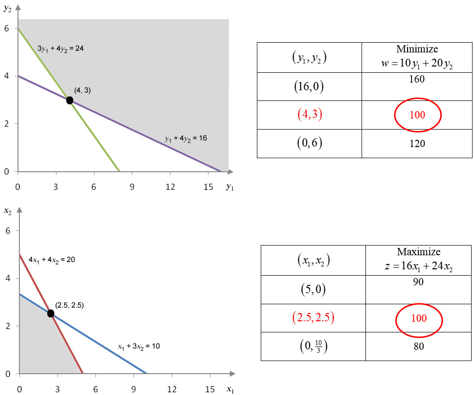
Let’s look at the solution of each linear programming problem graphically. For each problem, let’s look at a graph of the feasible region and a table of corner points with corresponding objective function values. From the table, we see that the solutions share the same objective function value at their respective solutions.

Although the corner points yielding the maximum or minimum are not the same, the value of the objective function at the optimal corner point is the same, 100. In other words,

Another connection between the dual problems is evident if we apply the Simplex Method to the dual maximization problem

If we rearrange the objective function and add slack variables to the constraints, we get the system of equations

This system corresponds to the initial simplex tableau shown below. The pivot column is the second column and the quotients can be formed to yield

The pivot for this tableau is the 3 in the first row, second column. If we multiply the first row by ¹/₃, the pivot becomes a 1 and results in the tableau

The first simplex iteration is completed by creating zeros in the rest of the pivot column. To change these entries, multiply the first row by -4 and add it to the second row. Then multiply the first row by 24 and add it to the third row.

Now that the pivot is a one and the rest of the pivot column are zeros, look at the indicator row to see if another Simplex Method iteration is needed. Since the entry in the first column of the indicator row, -8, is negative, we make the first column the new pivot column.

The quotients for each row of the tableau are formed below:

The smallest ratio is in the second row. The pivot, ⁸/₃, must be changed to a 1 by multiplying the second row by ,

Once the pivot is a one, row operations are used to change the rest of the pivot column to zeros.

The entry in the first row of the pivot column is

changed to a zero by placing the sum –¹/₃ of times the second row and the first row in the first row. The entry in the third row of the pivot column is changed to a zero by placing the sum of 8 times the second row and the third row in the third row,

Since the indicator row no longer contains any negative entries, we have reached the final tableau. If we examine the final simplex tableau carefully, we can see the solution to the standard maximization problem and the standard minimization problem:

The final simplex tableau gives the solution to the standard maximization problem and the solution to the corresponding dual standard minimization problem. This means that as long as we can solve the standard maximization problem with the Simplex Method, we get the solution to the dual standard minimization problem for free. This suggests a strategy for solving standard minimization problems.

Example 3    Find the Optimal Solution

In Section 4.2, we solved the linear programming problem

using a graph. In Example 2, we found the associated dual maximization problem,

Apply the Simplex Method to this dual problem to solve the minimization problem.

Solution In Example 1 and Example 2 we wrote this problem as a standard minimization problem and found the dual maximization problem. In this example, we’ll take the dual problem,

and apply the Simplex Method.

The initial simplex tableau is formed from the system of equations

Notice that the slack variables s₁ and s₂ are included in the equations corresponding to the constraints, and the objective function has been rearranged appropriately.

The initial tableau is

The most negative entry in the indicator row is -32, so the second column is the pivot column. Now calculate the quotients to find the pivot row,

The smallest quotient corresponds to putting the pivot in the second row, second column. To change the entry in this position to a one, multiply the second row by ¹/₄:

To put zeros in the rest of the pivot column, we utilize more row operations.

Since the indicator row is non-negative, this tableau corresponds to the optimal solution. The solution is found in the indicator row under the columns for the slack variables. The lowest value for w is 8 and occurs at (y₁, y₂) = (0, 8).

How is the standard minimization problem related to the dual standard maximization problem?

At this point, the connection between the standard minimization problem and the standard maximization problem is not clear. Let’s look at an example of a standard minimization problem and another related standard maximization problem.

The linear programming problem

is a standard minimization problem. The related dual maximization problem is found by forming a matrix before the objective function is modified or slack variables are added to the constraints. The entries in this matrix are formed from the coefficients and constants in the constraints and objective function:

To find the coefficients and constants in the dual problem, switch the rows and columns. In other words, make the rows in the matrix above become the columns in a new matrix,

The values in the new matrix, called the transpose, help us to form the constraints and objective function in a standard maximization problem:

Notice the inequalities have switched directions since the dual problem is a standard maximization problem and the names of the variables are different from the original minimization problem. Putting these details together with non-negativity constraints, we get the standard maximization problem

This strategy works in general to find the dual problem.

Example 2    Find the Dual Maximization Problem

In Example 1, we rewrote a linear programming problem as a standard minimization problem,

Find the dual maximization problem associated with this standard minimization problem.

Solution The dual maximization problem can be formed by examining a matrix where the first two rows are the coefficients and constants of the constraints and the last row contains the coefficients on the right side of the objective function.

In the case of this standard maximization problem, we get the 3 x 3 matrix

The vertical line separates the coefficients from the constants, and the horizontal line separates the entries corresponding to the constraints from the entries corresponding to the objective function. Notice that the entries are written before introducing slack variables or rearranging the objective function. The zero in the last column corresponding to the objective function comes from the fact that the objective function has no constants in it.

The coefficients and constants for the dual maximization problem are formed when the rows and columns of this matrix are interchanged. The new matrix,

is utilized to find the dual problem. The first row corresponds to the constraint ¹/4 x₁ + 7x₂ ≤ 4. The second row corresponds to the constraint x₁ + 4x₂ ≤ 1. Notice that each constraint includes a less than or equal to ( ≤ ) to insure it fits the format of a standard maximization problem. The last row corresponds to the objective function z = 2x₁ + 32x₂.

These inequalities and equations are combined to yield the standard maximization problem

What is a standard minimization problem?

In Section 4.3, we learned that some types of linear programming problems, where the objective function is maximized, are called standard maximization problems. A similar form exists for another for linear programming problems where the objective function is minimized.

The standard minimization problem is written with the decision variables y₁, … , y_n, but any letters could be used as long as the standard minimization problem and the corresponding dual maximization problem do not share the same variable names.

Often a problem can be rewritten to put it into standard minimization form. In particular, constraints are often manipulated algebraically so the each constraint has the form e₁ y₁ + e₂ y₂ + … + e_n y_n ≥ f. Example 1 demonstrates how a constraint can be changed to put it in the proper form.

For the problems in this section, we will require the coefficients of the objective function be positive. Although this is not a requirement of the Simplex Method, it simplifies the presentation in this section.

Example 1    Write As A Standard Minimization Problem

In Section 4.2, we solved the linear programming problem

using a graph. Rewrite this linear programming problem as a standard minimization problem.

Solution In a standard minimization problem, the objective function must have the form w = d₁ y₁ + d₂ y₂ + … + d_n y_n where d₁, … , d_n are real number constants and y₁, … , y_n are the decision variables. The objective function matches this form with .

Each constraint must have the form e₁ y₁ + e₂ y₂ + … + e_n y_n ≥ f where e₁, … , e_n and f are real number constants. Additionally, the constant f must be non-negative. The second constraint, 7y₁ + 4y₂ ≥ 32, fits this form perfectly.

The first constraint appears to have the correct type of terms, but variable terms are on both sides of the inequality. To put in the proper format, add ¹/₄ y₁ to both sides of the inequality:

¹/₄ y₁ + y₂ ≥ 2

With this change, we can write the problem as a standard minimization problem,

In addition to adding and subtracting terms to a constraint, we can also multiply or divide the terms in a constraint by nonzero real numbers. However, remember that the direction of the inequality changes when you multiply or divide by a negative number. This can complicate or even prevent a linear programming problem from being changed to standard minimization form.

How do you find the optimal solution for an application?

The Simplex Method can be applied to the brewery application developed earlier in the chapter.

Example 4    Find the Optimal Production Level

The linear programming problem for the craft brewery is

where x₁ is the number of barrels of pale ale, and x₂ is the number of barrels of porter. Use the Simplex Method to find the production level that maximizes profit.

Solution In Example 1, we added slack variables and found the initial simplex tableau for this standard maximization problem.

The initial simplex tableau is a 4 x 7 matrix,

The most negative entry in the indicator row is -100. This entry means the pivot column is the first column in the tableau. The quotients formed from the last column and the pivot column,

indicate that the third row is the pivot row.

The third row must be multiplied by ¹/_23.8  to change the pivot to a 1.

The entries in the first six columns are shown rounded to three decimal places when necessary, and the entries in the last column are rounded to the nearest tenth.

Now we need to use three row operations to place zeros in the rest of the pivot column.

The negative number in the indicator row tells us that the second column will be the new pivot column.

To locate the new pivot, form the quotients with the last column and second column. The quotients for the individual rows are

The numbers shown in the quotient are rounded numbers, and the amount calculated is rounded to the nearest integer. This does not affect our choice of the pivot row. If the quotients are close to each other, carry more decimals so you do not choose the wrong pivot row due to rounding. The new pivot is 0.544 in the first row, second column.

The new pivot is changed to a 1 by multiplying the first row of the tableau by ¹/_0.544:

We use three row operations to put zeros in the rest of the pivot column:

Since there are no negative numbers in the indicator row, we can read the solution from this tableau. If we cover the nonbasic variables s₁ and s₂,we see that the solution corresponding to this tableau is (x₁, x₂) = (35,328.2, 14,671.8) and P = 4,706,563.7 or approximately 35,328 barrels of pale ale and 14,672 barrels of porter for a maximum profit of about $4,706,564.

Example 3 and Example 4 both have two decision variables and were also done graphically in Section 4.2. In the next example, we apply the Simplex Method to a problem with three decision variables. Problems with more than two decision variables are impossible to do with the graphical methods introduced in Section 4.2.

Example 5      Find the Optimal Investment Portfolio

Investing in stocks and mutual funds are a trade off. We want to maximize the money we make from investments, but manage the risk of losing money in poor investments. Typically, investments with higher returns are riskier, and investments with lower returns are less risky.

Investors use several statistics to quantify the returns on their investments. For instance, websites such as Yahoo Financial calculate measures like average rate of return. This number indicates the investor’s total returns on an investment annualized over some time period. The higher the average rate of return, the more gains you achieve from dividends or the sale of the stock or mutual fund.

There are also several measures of risk available to investors. One commonly used indicator is called beta. The beta of a stock or mutual fund is calculated using regression analysis. The details of the analysis are not important for our purposes. However, understanding what the beta tells you is an important investing tool.

A stock or mutual fund’s beta measures the volatility of the investment’s price with respect to some benchmark like the S & P 500 or the Dow Jones Industrial Average. A beta of 1 indicates that the investment’s price will change with the benchmark’s changes. A beta less than 1 indicates that the investment’s price is less volatile than the benchmark. In other words, changes in the benchmark will be larger than changes in the investment’s price. A beta greater than 1 indicates that the investment’s price is more volatile than the benchmark. In this case, changes in the benchmark will be smaller than changes in the investment’s price.

Suppose an investor is interested in investing in three different mutual funds. The funds, their five year average annual return, and beta values are shown (as of July 31, 2010) in the table below:

The fund TIIRX has the highest rate of return and the lowest beta. The fund TCMVX has the lowest rate of return and the highest beta. On the surface, it would appear that the investor should put all of their money in TIIRX since that would yield the highest return and the lowest risk.

Each investor has their own requirements for their investments and in this case, the investor wants to diversify their holdings. This means the investor wants to lower their overall risk by investing in several broad categories of stocks. TIIRX seeks to invest 80% of its funds in securities which offer long term returns. It invests approximately 20% in smaller companies that offer an opportunity at growth. While this may seem like a good mix, the investor wishes the sum of what is invested in TCMVX and TIERX to be at least 25% of what is invested in TIINX.

If the investor has $100,000 to invest and wishes the average weighted beta to be no larger than 1, how much should the investor put in each of the three funds so that their returns are maximized?

Solution A good starting point for linear programming problems is the variables. In this problem, we want to find the amount of money to invest in each fund. It makes sense to define the variables as follows:

M: amount of money invested in Mid Cap Value Fund.
G: amount of money invested in Growth & Income Fund.
E: amount of money invested in International Equity Fund

We wish to maximize the return on the investment. The return on an investment is found by multiplying the amount invested by the average annual return. Since M, G, and E represent the amounts of money invested, 0.0172M, 0.0288G, and 0.0267E represent the return on these amounts. The objective function is the sum of these amounts or

where R is the total return.

Three pieces of information can help us to write out constraints. First, the investor has $100,000 to invest. This means the sum of the amounts invested in each fund must be less than or equal to 100,000 or

Second, the investor wishes the sum of what is invested in the Mid Cap Value Fund and International Equity Fund to be at least 25% of what is invested in Growth & Income Fund. Focusing on the word “sum” and the phrase “25% of”, we write

The word “sum” indicates that we must add the two quantities and the phrase “25% of” indicates that we must multiply the quantity by 0.25.

The final piece of information dictates that the investor “wishes the average weighted beta to be no larger than 1”. A weighted average tells us that we need to add up some terms and then divide by a total amount. The weighted sum of the risk is written as 1.16M + 0.93G + 1.04E. The term “weighted” indicates the presence of the variable in each term. If we had simply added up the beta values, they would have each contributed “equally” to the sum since each one appears in their own term. By multiplying the beta value by the amount invested in the corresponding fund, we are weighting the beta by the amount invested. If we do this, then a fund with a large amount in it will contribute more to the sum than a fund with very little invested in it. To average the weighted sum, we divide by the total amount invested or M + G + E. The constraint

reflects the investor’s wish that the average weighted beta be no more than 1.

If we add non-negativity constraints, the linear programming problem becomes

This linear programming problem is not in standard maximum form since the second and third constraints do not have the form

b₁ x₁ + b₂ x₂ + … + b_n x_n ≤ c

where b₁, b₂, … and c are real numbers and c ≥ 0. A little algebra changes these constraints to the proper form.

If we start with the second constraint and subtract M and E from both sides, we get the inequality

0 ≥ 0.25G – M – E

Flip the inequality and rearrange the order of the terms to yield

–M + 0.25G – E ≤ 0

This inequality has the proper form.

If we start with the third inequality and multiply both sides by M + G + E we are left with

1.16M + 0.93G + 1.04E ≤ M + G + E

Collect all of the terms on the left side to yield

0.16M – 0.07G + 0.04E ≤ 0

With these modifications, we can write out a standard maximization problem:

Now that the problem is in standard form, we can add slack variables to the constraints and write out the initial simplex tableau.

The objective function must be rewritten with all terms on the left side of the equal sign or

-0.0172M – 0.0288G – 0.0267E + R = 0

Notice that the variables are written in a particular order. Since the terms will match with columns in the tableau, we need to use this order for each equation we write.

Add the slack variables s₁, s₂, and s₃ to the inequalities

to give the equations

Combine these equations with the equation from the objective function to give

From this initial simplex tableau we need to pick a pivot column and row. To find the pivot column, locate the most negative entry in the indicator row at the bottom. The entry -0.0288 is the most negative entry so the second column is the pivot column.

The quotients for picking the pivot row are found by dividing the entries in the last column by the corresponding entries in the pivot column,

Remember that quotients with a negative numerator or denominator are ignored so the quotient for the third row isn’t even computed. The second row contains the smallest quotient, so the pivot is 0.25 in the second row, second column.

To change the pivot to a 1, multiply the second row by ¹/_0.25 or 4:

With the pivot changed, row operations are needed to change the other numbers in the pivot column to zeros.

After the first Simplex Method iteration, there is still a negative number in the indicator row. This tableau does not correspond to an optimal solution so we must select the first column as the pivot column and determine the new pivot row. Only the first row has an admissible quotient. The 5 in the first row, third column will be the new pivot.

To change the pivot to a 1, multiply the first row by ¹/₅:

Row operations are required to change the rest of the column into zeros.

After the row operations, there are no negative numbers in the indicator row. Covering the first, fourth and fifth columns, we can read off the solution (M, G, E) = (0, 80,000, 20,000) and R = 2838. Remember, by covering the first column we are assuming that M = 0.

The optimal solution is to invest no money in the Mid Cap Value Fund, $80,000 in the Growth & Income Fund, and $20,000 in the International Equity Fund. This combination of investments results in the largest return of $2838.

Even with more variables, the Simplex Method allows the standard maximization problem to be solved. Adding more decision variables or constraints simply adds more columns or rows to the initial simplex tableau. Although this makes for more writing, it does not change how the Simplex Method is applied.