Category: Finite Mathematics Ebook

What is a matrix inverse?

There are several matrices that are frequently used in mathematics. The identity matrix and the inverse matrix are two matrices that are related to each other. Each of these matrices is a square matrix meaning that they have the same number of rows as columns.

When referring to an identity matrix, we typically include the size unless the size is obvious from the context. For example, the matrix

is a 2 x 2 identity matrix.

The matrix

is a 3 x 3 identity matrix. If the size of the identity matrix is not clear from the context, a subscript is often used to indicate the size. For instance, a 4 x 4 identity matrix would be called I₄ and written

If an arbitrary square matrix is multiplied by an identity matrix and the multiplication is defined, the product is the arbitrary square matrix. The identity matrix identifies the matrix being multiplied.
We can write this symbolically for an arbitrary matrix A,

AI = IA = A

as long as the products can be carried out. To ensure the multiplication is defined, the identity matrix used must have the same size as the square matrix being multiplied.

Example 1      Multiply by an Identity Matrix

For the matrix

show that AI = IA = A.

Solution Start by multiplying the 2 x 2 matrix A by the 2 x 2 matrix I. Since the number of columns in A is 2, the number of rows in I must also be 2. In this case we can carry out this matrix multiplication and the result is a 2 x 2 matrix equal to A.

We can also compute in a similar manner:

Two square matrices that are inverses share a special property. The product of inverse square matrices is the identity matrix I with the same size.

Invertible matrices are matrices for which an inverse may be found. We make this distinction because some square matrices do not have inverses. Matrices that do not have inverses are called singular matrices.

In the next two examples, we determine if two matrices are inverses of each other by carrying out the products and to see if they are both equal to the identity matrix.

Example 2      Are Two Matrices Inverses?

If  and , are the matrices A and B inverses?

Solution For two matrices to be inverses, AB = BA = I. Let’s compute each product to see if they are equal to the identity matrix.

This product is equal to the 2 x 2 identity matrix. Let’s look the other product.

Both products are equal to the 2 x 2 identity matrix so the matrices A and B are inverses. We emphasize this fact by saying

Example 3      Are Two Matrices Inverses?

If  and , are A and B inverses?

Solution Compute the products AB and BA to determine if they are equal to the identity matrix. In both cases, the product of two 3 x 3 matrices is another 3 x 3 matrix.

Both products are equal to the 3 x 3 identity matrix. so

How do you interpret the entries in a product of two matrices?

Befre attempting to compute or interpret what the product tells you, it is instructive to determine the size of the product. As indicated earlier, the product of an m x k matrix and a k x n matrix is an m x n matrix. Once we know the size of the product, we can compute each of the entries in the product. The entries in the product are formed by corresponding the rows and columns in the factors, multiplying the entries, and summing the results. This operation is often very useful in computing various quantities in business. However, it is often not obvious exactly what the product tells you.

In a typical application, we can use the labels on the number of rows m in the first matrix to label the rows of the product. To label the columns in the product, write out the calculation for the first entry with the units on each factor. By analyzing the units, we can deduce what that entry tells us. The other entries will have a similar interpretation to the first entry.

Example 3      Interpret the Product of Two Matrices

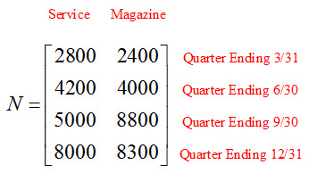
The number of new subscriptions by quarter is given by the matrix

New subscriptions may come from a subscription service or may come from the magazine’s marketing. The columns of N indicate the number of subscriptions from each source.

Find and interpret the product

Solution In this product we are multiplying a 4 x 2 matrix times a 2 x 1 matrix. Since the number of columns (2) in the first matrix matches the number of rows in the second matrix (2), we can carry out the matrix multiplication. The resulting product will be a 4 x 1 matrix:

Notice that each entry in the product is simply the sum of the entries on the same row in the first matrix. Since these values are the number of new subscriptions in that quarter, the sum in the product corresponds to the total number of new subscriptions in that quarter.

For instance, in the first quarter a total of 5200 new subscriptions were received from the subscription service and the magazine’s marketing efforts,

The numbers in the second matrix have no units. The effect of multiplying by the matrix  is to add the entries in each row of the matrix N.

Example 4      Interpret the Product of Two Matrices

The new subscriptions described by the matrix

contribute different amounts of cash to Ed Magazine. Subscriptions enlisted by the subscription service pay $10 for a subscription, but only $2 goes to the magazine. Subscriptions developed through the magazine’s marketing campaigns pay $12 and all of this cash goes to the magazine. We can summarize this information in the matrix

Find and interpret

Solution Let’s check the size of each matrix to insure that the matrix multiplication is possible.

The number of columns in N representing the number of new subscriptions and the number of rows in S representing the cash from subscriptions are both equal to 2 so the multiplication can be carried out to give a 4 x 1 product.

We can form the entries in the product by corresponding the rows in N with the column in S:

The four rows in the product correspond to the four quarters, but what do the entries tell us about those quarters?

To answer this question, let’s look at the first entry in detail:

Each term has units of dollars and indicates the amount of cash received from the sales of subscriptions to new subscribers of each type (from the subscription service and from the magazine’s promotions). So the sum, 34400 dollars, represents the total amount of cash received from both types of subscribers together.

Other entries can be analyzed similarly to show the total cash received from new subscribers in the other three quarters.

How do you multiply two matrices?

The process of multiplying matrices is different from scalar multiplication or the other matrix operations in the previous section. Instead of multiplying corresponding entries, in matrix multiplication we multiply the rows in one matrix by the columns in another matrix. This process can be demonstrated by multiplying a row matrix times a column matrix. Suppose we have a 1 x k matrix,

and a k x 1 matrix,

In each matrix, the dots help to indicate the arbitrary number of rows or columns in each matrix. Although this number k is arbitrary, the number of columns in A must match the number of rows in B. Otherwise it is not possible to carry out the multiplication process.
To find the product these matrices, we must multiply the entries in the row matrix by the entries in the column matrix and add the resulting products:

Notice that each product comes from corresponding columns and rows. In other words, the first product is formed from the first column in the first matrix and the first row in the second matrix, the second product is formed from the second column in the first matrix and the second column in the second matrix, and so on.

Let’s try the following product:

To help identify the factors in the products, let’s color code each corresponding factor and carry out the sum:

The key to carrying out the process is to correspond the factors in each product correctly.

This process is carried out several times when matrices with more than one row or column are multiplied. However, the number of columns in the first matrix must match the number of rows in the second matrix.

Example 1    Multiply Two Matrices

Let

Find the products indicated in each part.

a.  AB

Solution To be able to compute this product, the number of columns in A must equal the number of rows in B. Since A has 3 columns and B has 2 rows,

it is not possible to compute this product.

b.  BA

Solution For this product, the number of columns in B is equal to the number of row in A,

This means the product can be computed. The size of the resulting product is determined by the number of rows in B, 2, and the number of columns in A,3:

Now that the size of the product is known, we can find the entries in the product.

Start with blank entries in a 2 x 3 matrix:

We can find the value of any entry in the product by corresponding the proper row and column in the factors. For instance, the entry in the second row, first column is computed from the second row of the first matrix and the first column of the second matrix:

This entry is placed in the product matrix,

The entry in the first row, third column is computed from the first row of the first matrix and the third column of second column:

Adding this entry to the product matrix yields

We can compute the other four entries in the product matrix similarly.

Example 2    Multiply Two Matrices

The table below gives the number of expiring subscriptions for Ed Magazine.

This information is summarized in the matrix

The different categories of subscribers renew their subscriptions at different rates. Twenty five percent of the first time subscribers renew their subscriptions and fifty percent of the existing subscribers renew their subscriptions.

a. Use matrix multiplication to find a matrix describing the total number of renewed subscribers by quarter.

Solution To see how matrix multiplication can be used to calculate the total number of renewed subscribers, watch the video, let’s look at the quarter ending 3/31. In that quarter, 6000 first time subscribers and 15000 continuing subscribers have their subscriptions expiring. We know that 25% of the first time subscribers will renew and 50% of the continuing subscribers will renew.

The total number of renewed subscriptions in the first quarter is

We can also calculate the total number of renewed subscriptions in other quarters using this same strategy.

Notice that each number is the sum of two products. The product of two matrices creates a new matrix where each entry is a sum of products. This suggests that we define a matrix

of the renewal rates for the subscribers groups.

The product

can be carried out since E has 2 columns and P has 2 rows.

The resulting product is a 4 x 1 matrix:

Notice that each entry matches the totals found earlier. Using matrices we are able to compute the total number of renewals by quarter efficiently. Additionally, if more quarters are included in E the process can still be carried out by adding more rows to E.

b. A renewing subscriber pays $18 per year for a subscription. Find a matrix that gives the cash receipts from renewed subscriptions by quarter.

Solution The product EP gives the total number of renewed subscriptions by quarter. To find the cash receipts from these subscriptions, we must multiply each entry in the product by 18. Multiplying the product EP by the scalar 18 gives

c. The matrix

gives the cash receipts from new subscriptions by quarter. Find the matrix R that gives the total cash receipts from new and existing subscriptions.

Solution The total cash receipts R is the sum of cash receipts from new subscriptions R₁ and cash receipts from existing subscriptions R₂,

Combine R₁ and R₂ to yield

How do you graph a system of linear inequalities?

A craft brewery cannot produce unlimited amount of beer each month. As we have seen in this section, there are constraints on the amount of beer that can be fermented as well as the amounts of each ingredient that can be shipped to the brewery and stored on site. If barrels of pale ale and barrels are produced per month,

Together these inequalities define possible combinations that the brewery may produce. In addition, it does not make sense for the amount of beer produced to be negative. So in addition to these inequalities, we also require that

Together these inequalities form a system of linear inequalities.

A system of linear inequalities is two or more linear inequalities solved simultaneously. Each linear inequality has a solution that is a half plane. The solution set of the system of linear inequalities is all ordered pairs that make all inequalities in the system true. If we examine the solutions sets of each of the individual inequalities together, the solution set of the system of inequalities is where all of the individual solution sets overlap.

Example 4    Graph the System of Linear Inequalities

Graph the solution set for the system of linear inequalities

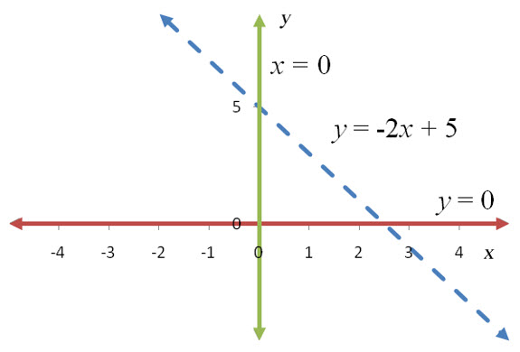
Solution To get started, we need to graph the equations y = -2x + 5, x = 0, and y = 0. The first equation will be graphed as a dashed line since the corresponding inequality is a strict inequality. The vertical line x = 0 and horizontal line y = 0 will be graphed as solid lines since the corresponding inequalities include an equal sign.

Figure 12 – The corresponding equations for the inequalities in Example 4.

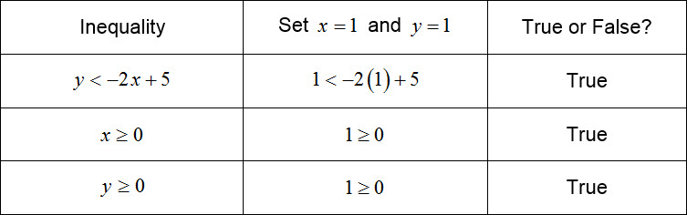
With these boundary lines in place, we need to test a point in each inequality to know the individual solution for each inequality. It is not possible to use (0, 0) since it lies on the horizontal and vertical lines.

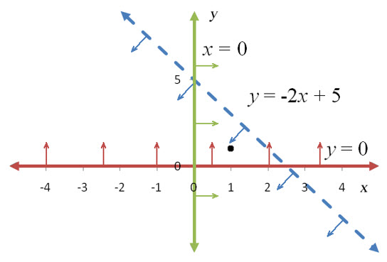
Another point that is easy to test is (1, 1).

For each line, place arrows on the lines indicating which side is a part of the solution. Since the test point is true in each inequality, we need to place arrows on each line pointing toward the test point.

Figure 13 – The arrows on each line point in the direction of the black test point since it makes each inequality true.

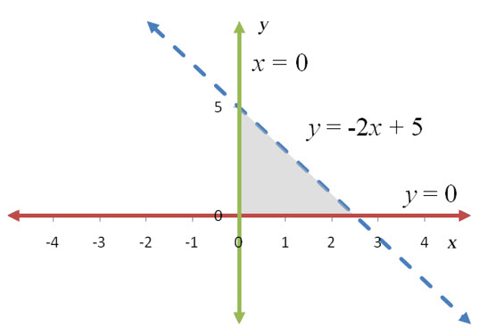
Any point in the triangular region where (1,1) lies will make all of the inequalities true. In any other part of the graph, one or two of the inequalities might be true, but not all three in the system. Shade the triangular region where all of the individual solutions overlap to give the graph in Figure 14.

Figure 14 – The solution to the system of linear inequalities. Any ordered pair in the gray shaded region makes all three inequalities true.

When the solution set to a system of inequalities can be enclosed in a circle, the solution is bounded. The solution in Example 4 is an example of a bounded solution set.

Example 5    Graph the System of Linear Inequalities

Graph the solution set for the system of inequalities

Solution In this example, subscripted variables are used. This makes it harder to pick an independent variable. Either variable can be the independent variable. For no particular reason, we’ll graph x₁ on the horizontal axis and x₂ on the vertical axis.

This system includes the non-negativity constraints x₁ > 0 and x₂ > 0. These tell us that the solution must lie in a quadrant where all variables are not negative. We can simplify the example by realizing that this is in the first quadrant. By graphing all of the lines primarily in the first quadrant, we can speed up the graphing process.

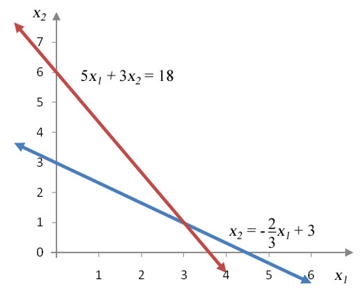
To graph the other two constraints, we need to graph the lines that form the border of the solution set,

The first equation is in slope-intercept form with a slope of –²/₃ and a vertical intercept of 3. Drawing a line through (0, 3) with a slope of –²/₃ gives the border of the first constraint.

The second line is easy to graph if we find the intercepts. If we set x₁ = 0, we get x₂ = 6 yielding the vertical intercept . The other intercept is located by setting x₂ =0. The resulting equation can be solved for x₁ to yield the horizontal intercept (x₁, x₂) = (¹⁸/₅, 0).

Figure 15 -The borders of the first two inequalities in Example 5. The graph is drawn in the first quadrant due to non-negativity constraints.

Drawing a line through these two ordered pairs results in the border for the second constraint. Both lines must be drawn with a solid line since both constraints include an equal sign in the inequality.

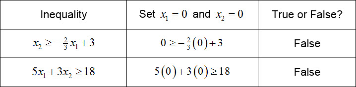
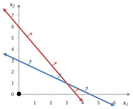
Now pick a test point like (0, 0)  to determine which side of each line should be shaded.

Each inequality is false at the test point so the solution set to each inequality must be on the side of the line where the test point is not located. Use arrows on each line to indicate the side of each line where the test point is not located.

Figure 16 -For each inequality, the side opposite the test point must be shaded since the inequalities are both false at the test point.

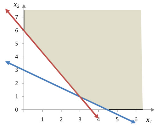
The solution set to the system is all of the ordered pairs in the first quadrant (due to the non-negativity constraints) that are solutions to each of the inequalities in the system. By noting where the solution sets for each inequality overlap, we get the solution set below.

Figure 17 – The solution set to the system in Example 5.

Because this solution set extends infinitely far, the region cannot be enclosed in a circle. Solution sets that cannot be enclosed in a circle are called unbounded solution sets.

Example 6    Graph the System of Linear Inequalities

Graph the solution set for the system of inequalities

Solution The border of the solution set is formed by

The first equation is a line in slope-intercept form with a slope of 1 and a vertical intercept of 3. This line is graphed as a solid line since an equal sign is part of the inequality.

The second equation can be solved for y to yield y = x. This is a line with a slope of 1 that passes through the origin. Since the inequality is a strict inequality, the border is graphed with a dashed line.

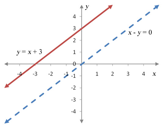
Figure 18 – The borders of the inequalities in Example 6.

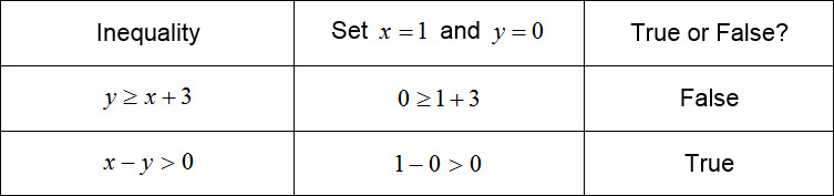
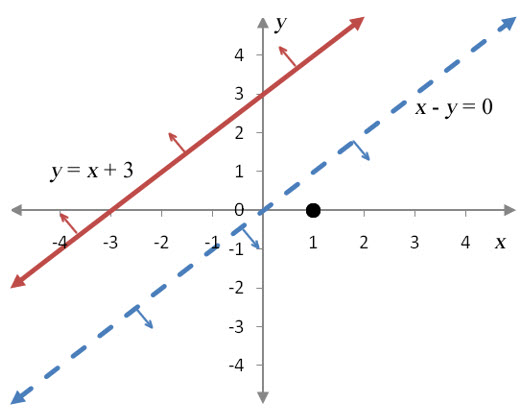
 The border of the second inequality passes through the ordered pairs (0, 0) and (1, 1), the ordered pairs we have used in other examples as test points. For this example, we’ll use (1, 0) as the test point.

Figure 19 – The borders of the inequalities with arrows indicating the individual inequality solution. The first inequality is false at the test point so the side opposite is the solution. For the second inequality, the inequality is true at the test point so that side is the solution for the inequality.

As with previous examples, the solution set of the system of inequalities is where all of the individual inequality solution sets overlap. Examining the graph carefully, we note that there is no place on the graph where all of the inequalities overlap. There are no ordered pairs that satisfy all of the inequalities simultaneously, so there are no solutions to the system of inequalities.

Now that we’ve tried out the strategy for solving several simple systems of inequalities, let’s revisit the system of inequalities for the craft brewery.

Example 7    Graph the System of Inequalities for the Craft Brewery

The system of inequalities for a craft brewery is

where x₁ is the number of barrels of pale ale produced, and x₂ is the number of barrels of porter produced. Graph the system of inequalities with as the independent variable.

Solution The non-negativity constraints restrict the solution to the first quadrant. Because of this, we’ll restrict the borders of the other three inequalities to this quadrant and not extend any shading of the final solution beyond the first quadrant.

The borders of the inequalities for capacity, malt, and hops are given by the equations

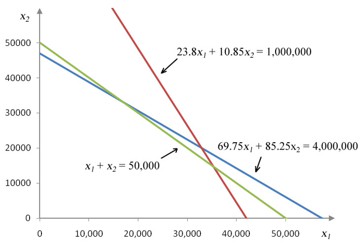
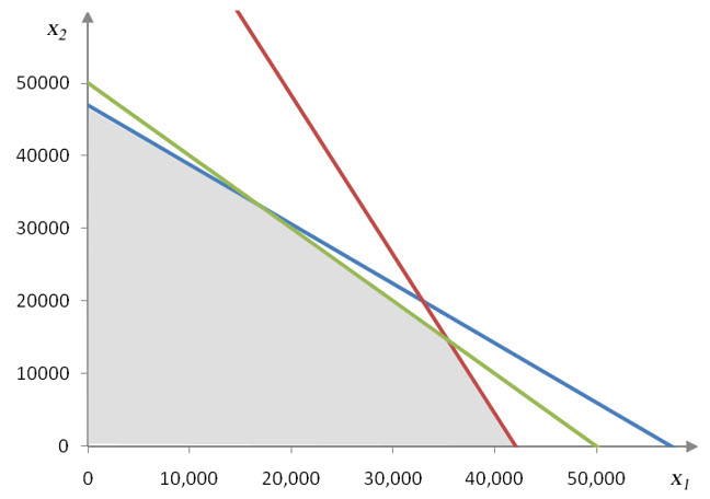
Figure 20 – The borders of the inequalities in Example 7.

Each of these equations was graphed earlier in this section. Putting all of the lines on a single graph yields the graph in Figure 20.

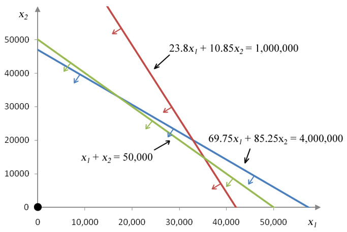
To find the solution sets of each of the inequalities, let’s test the ordered pair (0, 0) in each inequality and indicate shading with arrows in the graph.

Based on this table, the test point must be included in the solution set of each of the inequalities. The arrows on each of the lines must point to the half-plane containing the test point for each inequality.

Figure 21 – For each inequality, the test point must be included in the solution suggesting the shading on the graph.

The individual solution sets all overlap in a region that is to the left and below all of the lines.

Figure 22 – The region shaded in gray is the solution to the system of inequalities for a craft brewery. This region is where the solutions to all inequalities in the system coincide.

At any point in the solution set, the brewery can produce the number of barrels of beer indicated by the ordered pair and satisfy all of the constraints for capacity, malt and hops.

How do you graph a linear inequality?

To graph the solution to an inequality on a rectangular coordinate system, the inequality must contain only two variables. The craft brewery inequalities discussed above contained five variables since the brewery produced five different types of beer. Let’s simplify the inequalities to only two variables so that we can view the solutions to the inequality on a rectangular coordinate system. We’ll do this by modifying the number of beers a particular brewery produces.

Suppose a craft brewery has a monthly capacity of 50,000 barrels of beer and produces two styles of beer, a pale ale and a porter. If the brewery is not to exceed the monthly capacity, we know that

where x₁ is the number of barrels of pale ale produced each month, and x₂ is the number of barrels of porter produced each month.
Using and may seem confusing, but we could have easily written this same inequality as

where x is the number of barrels of pale ale produced each month, and y is the number of barrels of porter produced each month. The names of the variables are irrelevant. However, since we want to be able to generalize two variable problems to problems with more than two variables, we’ll stick with subscripts for this example.

When an inequality in two variables is graphed, we start by changing the inequality to an equation. The equation for this craft brewery is

We’ll graph this equation with x₁ on the horizontal axis (the independent variable) and x₂ on the vertical axis (the dependent variable). It is perfectly acceptable to switch the variables on the axes. The key is to pick an axis for each variable and to stick with it throughout the entire problem.
The easiest way to graph this equation is by using the intercepts. By setting each variable equal to 0, we can find the corresponding value for the other variable:

Drawing a line through these two points gives us the following graph:

Figure 3 – The line x₁ + x₂ = 50,000 passes through the intercepts at (0, 50,000) and (50,000, 0).

For every point on this line, the sum of x₁ and x₂ is 50,000. For instance, the point (25000, 25000) is on this line since . Points that are not on the line have a sum that is either greater than or less than 50,000. The line in the graph forms the border between points where the sum is greater than 50,000 and points where the sum is less than 50,000.

To determine which side is which, pick a convenient point on the graph that is not on the line. Test this point in the original inequality. If the inequality is true, then every point on the side of the line the test point comes from is in solution to the inequality. If the inequality is false when the test point is substituted, all points on the opposite side of the line from the test point are in the solution for the inequality. By shading the half plane where the test point is true, we can indicate all of the ordered pairs in the solution set of the inequality.

When the inequality includes an equal sign (like < or >) we draw the line separating the two half planes with a solid line. This tells us that the line corresponding to the border, x₁ + x₂ = 50,000, is included in the solution set of the inequality.

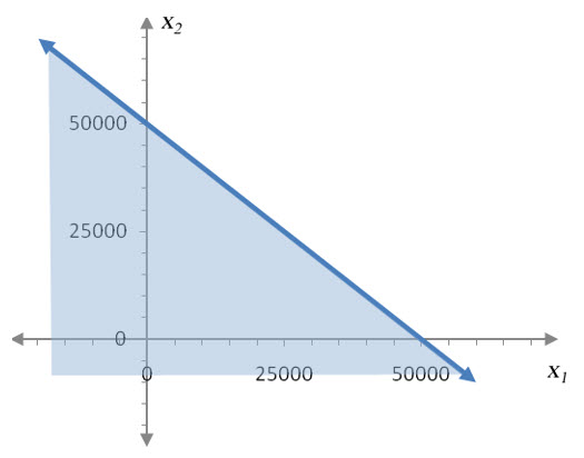
For the inequality , a convenient test point is (0, 0). Set x₁ = 0 and x₂ = 0 to yield 0 + 0 < 50,000. Since this is a true statement, all of the points on this side of the line satisfy the inequality. To show this graphically, we shade all of the points on that side in the graph and graph the border as a solid line.

Figure 4 – The solution set to x₁ + x₂ < 50,000 extends infinitely far below and to the left of the line and includes the line x₁ + x₂ = 50,000.

If the inequality is a strict inequality (with no equal sign), the line separating the two half planes is drawn with a dashed line. This tells you that the border is not included in the solution set. For instance, the solution set to the inequality x₁ + x₂ < 50,000 is shown in Figure 5.

Figure 5 – The solution set to x₁ + x₂ < 50,000 extends infinitely far below and to the left of the line and does not includes the line x₁ + x₂ = 50,000.

Example 1    Graph the Linear Inequality

Graph 15x + 20y < 300.

Solution This linear inequality uses two variables, x and y. We’ll choose x as the independent variable and y as the dependent variable. This means that the horizontal axis will be labeled with x, and the vertical axis labeled with y.

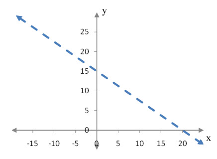
To graph the border between the two half planes, we need to graph 15x + 20y = 300. This is done by solving for y:

In slope-intercept form we recognize the slope, –³/₄, and vertical intercept, 15, and use them to graph the line. Since the inequality is a strict inequality, the line must be graphed as a dashed line.

For some equations it may be easier to find the intercepts of the equation:

Using the slope-intercept method or the intercept method, the graph of 15x + 20y = 300 looks the same.

Figure 6 – The line 15x + 20y = 300 is the border between half planes. Note the slope of the line and the intercepts. Either method gives the same line. Since the inequality is a strict inequality, the line will be drawn as a dashed line.

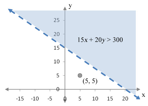
Any point that is not on the line can be the test point. We’ll test the point (5,5). Putting this ordered pair into the inequality yields

Since this ordered pair does not satisfy the inequality, shade the portion of the plane on the other side of the line from the test point.

Figure 7 – The solution set to 15x + 20y > 300 extends infinitely far above and to the right of the dashed line.

Example 2    Find and Graph the Linear Inequality

At a craft brewery, four different ingredients are combined to create beer. Yeast, malted grain, hops and water are mixed, cooked, and fermented in large kettles. The production of beer is limited by several factors. First, the size of the equipment limits the number of barrels that can be produced to 50,000 barrels per month. If x₁ barrels of pale ale are produced and x₂ barrels of porter are produced, we know that

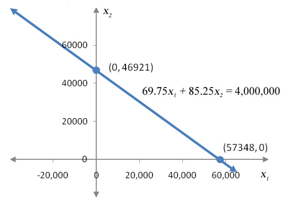
Production is also limited by the availability of grain, the capacity to ship grain to the brewery, and the storage capacity at the brewery. The brewery can process and store 4,000,000 pounds of malted grain per month. For each barrel of pale ale, the brewery uses 69.75 pounds of malted grain. For each barrel of porter, the brewery uses 85.25 pounds of malted grain.

Using this information, write and graph a linear inequality describing the total amount of malted grain used each month at the brewery.
Solution To write an inequality for the total amount of grain, we need to recognize that this brewery can use no more than 4,000,000 pounds of malted grain each month,

Malted grain is used in each of the two beers produced. The amount of grain used in the pale ale is found by multiplying the amount of grain used per barrel times the number of barrels of pale ale produced,

The units in these two factors reduce to yield overall units of pounds.

We can also determine the amount of grain in the porter by writing

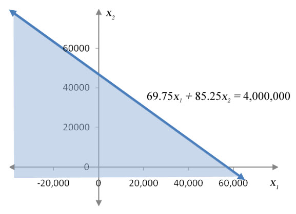
Combining the amount of grain in the pale ale, 69.75x₁, and the amount of grain in the porter, 85.25x₂, yields the inequality for the grain usage,

To graph this inequality, change the inequality to an equal sign,

and find the intercepts:

As before, we’ll graph this line with as the independent variable. We also use a solid line since the inequality includes an equal sign.

Figure 8 – The border for the inequality. The border is drawn with a solid line since the line is included in the solution set.

Pick a convenient test point like (0, 0) to see which side of the line is in the solution set.

If we set x₁ =0 and x₂ =0 in the inequality, we get

Since the test point at the origin makes the inequality true, shade the side of the line that includes the origin.

Figure 9 – The solution set for 69.75x₁ + 85.25x₂ < 4,000,000 extends infinitely far to the left and below the line.

Continue reading “Section 4.1 Question 1”