In this section you will look at systematic ways of counting objects. Although we start by simply listing out things and counting them, eventually we will be able to count things like possible four number pin codes without actually listing them all out.
We need to be able to count objects to be able to calculate probabilities. Probability is all about calculating how likely it is for an event to occur. On the surface this may seem a bit foreign, but you encounter probability on a daily basis. How often do you hear someone say “that the chances are 50-50”? Or that there is a “90% chance of rain”.
Both of the statements assign a number to a random occurrence. The numbers give you an idea of whether that event will actually occur. In this chapter you will learn what type of information is needed to assign these numbers and how you can utilize them to make decisions.
Our objectives for this section are to
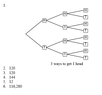
count elements in a set by listing all possibilities,
calculate the likelihood of an event by counting outcomes in the event and sample space,
distinguish between probability and odds.
Use the workbook and videos below to help you achieve these objectives.
Players in the National Basketball League (NBA) range from 5’9″ (Kay Felder) to 7’3″ (Boban Marjanović) with a mean of about 6’7″. If we compare this to players is the Women’s National Basketball League (WNBA), we see that heights range from 5’5″ (Leilani Mitchell) to 6’9″ (Brittney Griner). The mean in the WNBA is about 6′.
It is not surprising to see that the NBA has a greater mean since men are taller than women in general. However, is there more variation in height in the NBA or in the WNBA? TO answer this question, we need to calculate whether the men are farther from the mean and compare it to the same measure for women. This is precisely what the standard deviation measures…deviations from the mean.
In this section, you will learn how to
compute the range of a data set,
compute and interpret the standard deviation of a set of data.
compute and interpret the coefficient of variation for a set of data,
compute a five number summary of a set of data
interpret quartiles and percentiles,
construct a stem and leaf plot.
These measures will allow you to determine how spread out a set of data are.
Use the workbook and videos below to learn how to compute these measures of variation. Remember to complete the practice problems so that you can do these computations yourself.
When we are given a large set of data, it is difficult to look at it and get a meaning from it. In the graphic above, each state is color coded by its mean elevation. To calculate this information, thousands of pieces of data needed to be analyzed to determine what the central tendency for elevation was in each state. Examining the graphic, we se that the elevations in the western US are higher than in the eastern US. This trend would probably not have been obvious from the raw data.
In this section, we’ll begin to examine descriptive statistics. Descriptive statistics are numbers that are used to summarize the data. For this section, we’ll look at numbers which help us to determine the central tendency of a set of data. Our objectives for this section are to
Compute the mean, median and mode of data.
These measures will allow us to compare the central tendency in two different sets of data.
Use the workbook and videos below to learn how to compute these measures of central tendency. Make sure you work through the practice problems for computing these measures from raw data as well as frequency tables.