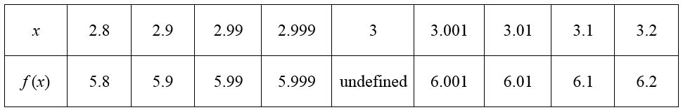
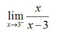
Suppose we have a rational function . We can examine the behavior of this function by constructing a table of values.
This function is undefined at x = 3 so we cannot find a function value there. However, we can find function values near x = 3.This table shows how the functions values change for different values of x near x = 3. In this table, x values on the left of 3 are in red. Values on the right side of 3 are in blue.
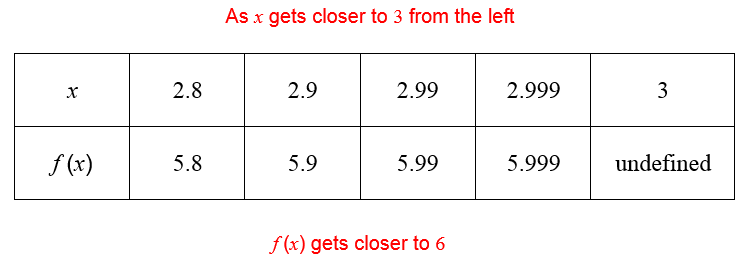
Let’s take a closer look at x values on the left side of x = 3.
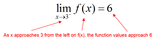
On the left side of 3, the function values get closer and closer to 6 as x gets closer to 3. Mathematically, we say that the limit as x approaches 3 from the left is 6. A limit represents the relationship between x and f (x) as x approaches some value.
This relationship is represented symbolically using the symbol lim.
We read this as, “the limit of f (x) as xapproaches 3 from the left is 6.” The value of the limit is determined by x values that are closer and closer to 3, not the value at x = 3. We will examine situations later in this section when we will use the value at a point to find the limit. In general, the value of the limit as x approaches some value is not equal to the value of the function at that xvalue. In the case of , the function is not even defined at x = 3.
A function f (x) has a limit L as x approaches a from the left, if the value of f (x) can be made arbitrarily close to L as x is made arbitrarily close to a from values on the left of a (but not equal to a). We symbolize this relationship by writing
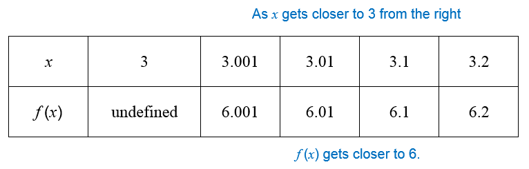
We can also evaluate a limit on the right side of on the function .
Based on this table, we see that as x gets closer and closer to 3 on the right, f (x) gets closer and closer to 6. This means that
The plus sign behind the x value indicates that we are approaching the value from the right side of 3. We read this as “the limit of f (x) as x approaches 3 from the right is 6.”
A function f (x) has a limit L as x approaches a from the right, if the value of f (x) can be made arbitrarily close to L as x is made arbitrarily close to a from values on the right of a (but not equal to a). We symbolize this relationship by writing
Example 1 Find a Limit Using a Table
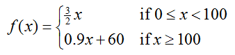
Let f (x) be the piecewise function
Use a table to find each of the limits below.
a.
Solution In this piecewise function, two expressions define the function. For x values in the interval [0, 100), the expression 3/2 x gives the y values for the function. We can use this expression to construct a table for values of x slightly to the left of x = 100.
As the x values in the table get closer and closer to 100, the corresponding f (x) values get closer and closer to 150. Based on this observation, we conclude that the left hand limit is
b.
Solution For x values in the interval [100, ∞), the expression 0.9x + 60 gives the yvalues for the function. This expression can help us to form the following table of values slightly to the right of x = 100.
As x values get closer and closer to 100, the values for f (x) get closer and closer to 150. The right hand limit is
c.
Solution Since the left hand and right hand limits are both equal to 150, the two-sided limit is also equal to 150,
Examples like the ones we have examined might lead you to believe that all limits are equal to some value. However, this is not always the case. In the next two examples, the limits do not exist.
Example 2 Find a Limit Using a Table
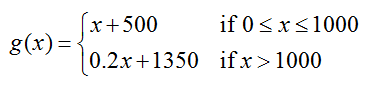
Let g(x) be the piecewise function
Use a table to find each of the limits below.
a.
Solution In this limit, x is approaching 1000 from values on the left. On this side of 1000, the function is defined by the expression x + 500. Let’s examine the behavior of this expression slightly to the left of 1000.
As x approaches 1000, the values of get closer and closer to 1500. This indicates that the left hand limit is
b.
Solution On the right hand side of 1000, the function is defined by the expression 0.2x + 1350. The table below shows values in that region.
Based on this table, as x approaches 1000 from the right, the function approaches 1550. Symbolically, we write
c.
Solution In the previous parts, we evaluated the limits from the left and right. Since the limit from the left is not equal to the limit from the left, the two-sided limit does not exist.
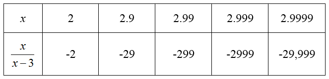
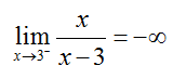
Example 3 Find a Limit Using a Table
Use a table to evaluate the limit
Solution Since this is a left hand limit, start by constructing a table of values slightly to the left of x = 3.
As x approaches 3, the value of the function gets more and more negative. Because the function is not approaching a value, we say that the limit does not exist.
Since it does the by growing large and negative, we write
For limits that do not exist and do it by becoming more and more positive, we write that the limit is equal to ∞. The infinity symbol always indicates that the limit does not exist because the values are becoming larger and larger.
The linear and quadratic functions we have introduced so far use a single rule to define the function. For a piecewise defined function, the function is defined by several rules. Each rule corresponds to a different piece of the function.
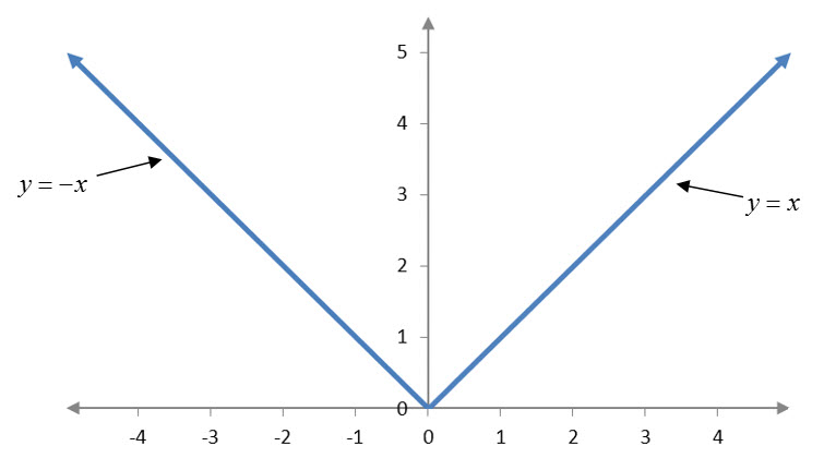
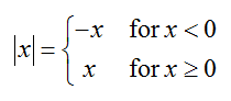
You are probably already familiar with one piecewise defined function. The absolute value function,
f (x) = |x|
appears to be a function that is defined by a single rule. However, if we look at the graph of the absolute value function, you see two different lines in the shape of a “v”.
Figure 4 – The absolute value function.
There are two pieces to the function. On the left side of x = 0, the function has a slope of -1 and a y-intercept of 0. On the right side of x = 0, the function has a slope of 1 and a y-intercept of 0. We can put this description together in a piecewise function as
Each line of the formula corresponds to a corresponding piece of the graph. To find an output from a piecewise function, we must determine which piece of the function the input belongs. For instance, the input x = -2 is in the top part of the function’s formula since this x value is less than zero. The output is
|-2| = -(-2) = 2
For a nonnegative input like x = 3, we find the output from the bottom part of the function’s formula,
|3| = 3
A piecewise function may have any number of pieces and may or may not be defined for every possible input. If there is no piece of the function defined for an input, we simply say the output is undefined.
Example 10 Piecewise Function
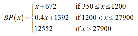
The Basic Plus Plan is a medical insurance plan offered by a self insured trust in Northern Arizona. The total annual cost (in dollars) to an insured person is
where x is the amount of medical charges incurred at the point of treatment.
a. Find the total annual cost for $5000 in medical charges.
Solution We must find the value of BP(5000). The input lies in the interval 1200 < x ≤ 27900 so the total annual cost is
BP(5000) = 0.4(5000) + 1392 = 3392
The total annual cost corresponding to $5000 in charges is $3392.
b. Find the total annual cost for $30,000 in medical charges.
Solution Medical charges of $30,000 lie in the third piece of the formula, so
BP(30000) = 12552
A person incurring $30,000 in medical charges would have a total annual cost of $12,552. In fact, for any amount of medical charges above $27,900. the total annual charge is $12,552. This is due to the fact that the plan has reached its out of pocket maximum at this level of charges.
c. Find the total annual cost for $250 in medical charges.
Solution No part of the function corresponds to so the output is undefined. The domain of the function is and this input lies outside of this interval.
Problems in business and finance are often mathematical in nature. These problems come from real-world situations that can be extremely complex. A mathematical model is a mathematical representation of the situation. Often these representations take the form of functions.
The price of a product may be constant or it may change in response to the quantity sold. If the quantity of some product sold increases, the price may decreases. A demand function displays the relationship between the price per unit P of a product and the quantity Q demanded by consumers. For example, the relationship for a certain product may be
P = -0.0002Q + 55
We say that the price P is a function of the quantity Q. By saying “function of quantity Q”, we are indicating that the independent variable is Q and the dependent variable is P. The same relationship can also be written as
Q = -5000P + 275000
Now the quantity Q is a function of the price P. This means that P is the independent variable and Q is the dependent variable.
Function notation is used to emphasize the independent variable in a function. Functions are named with a letter or phrase. Next to the name is a set of parentheses with the independent variable inside. For a demand function, we might use the letter Dto name the function. For the two equations above, we would write
D(Q) = -0.0002Q + 55 or D(P) = -5000P + 275000
Knowing what the independent variable is helps us to determine the input to and out from the function. For instance, if we need to find the price of the product when the quantity demanded is 10,000 units we would set Q = 10,000 in D(Q) = -0.0002Q + 55. We indicate this by writing
D(10000) = -0.0002(10000) + 55 = 53
In the function notation, each Q is set equal to 10,000. Since the input is a quantity, the output must be the corresponding price.
It may seem tedious to replace P with D(Q) to define a function. However, in many situations we need to work with two equations simultaneously. Without a name for the function, we would have a difficult time distinguishing the two formulas.
Example 6 Supply Functions
A supply function also displays the relationship between the price and the quantity of a product. Unlike the demand function, the supply function models the price P at which suppliers are willing to supply Q units of the product. Suppose this relationship is
P = 0.0001Q
a. Use function notation to define the supply function as a function of the quantity Q. Use the letter Sto name the function.
Solution Using the name S and the independent variable Q, the appropriate function notation is S(Q). The function definition is
S(Q) = 0.0001Q
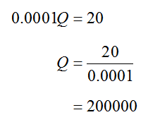
b. Use the function definition to find the price P at which suppliers would be willing to supply 20,000 units.
Solution Set in the function to yield
S(20000) = 0.0001(20000) = 2
At a price of $2 per units, suppliers would be willing to supply 20,000 units.
c. What does it mean for S(Q) = 20?
Solution When the function notation is set equal to a number, the output from the function is being given. In this case, the price is equal to $20. If we replace the function notation with its formula, we can solve the resulting equation to find the quantity Q corresponding to a price of $20:
At a price of $20 per unit, suppliers are willing to supply 200,000 units.
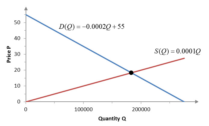
Typically, the demand and supply functions for a product are graphed together. Let’s put the two functions we have been using together.
Figure 3 – The equilibrium point is the point of intersection of the demand and supply functions.
On this graph, the two functions cross. At the point of intersection, the quantity that consumers are willing to buy is equal to the quantity that manufacturers are willing to supply. We can find this point algebraically by setting the two functions equal,
D(Q) = S(Q)
and solving the resulting equation for Q.
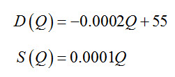
Example 7 Find the Equilibrium Point
The supply and demand functions for robotic hamsters are
Find and interpret the equilibrium point.
Solution The supply and demand are equal when
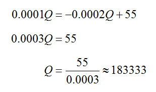
The price at this quantity may be obtained from either function. The equilibrium price is
At this price, the quantity demanded by consumers and the quantity manufacturers are willig to supply is approximately 183,333 robotic hamsters.
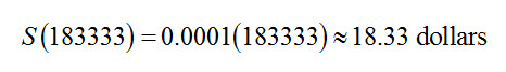
Businesses operate by obtaining money by the sales of goods and services. The amount of money obtained through the sales of goods and services is called revenue. Revenue is modeled by multiplying the quantity a good or service by the price of each unit of the good or service. We can write this model in mathematical form by writing
revenue = price per unit × quantity
In some situations, the price per quantity may be a constant. For the robotic hamsters, the price per quantity is given by the demand function D(Q). When we substitute the demand function into the revenue relationship, we get the revenue function,
R(Q) = D(Q) Q
We can form this function using the demand function.
Example 8 Revenue Function
The demand function for robotic hamsters is
a. Use function notation to define the revenue function for this application as a function of the quantity Q.
Solution We need to write a revenue function, R as a function of Q, R(Q). Using the revenue relationship, we find
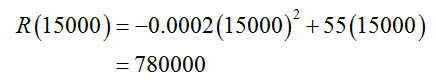
b. Use the function from part a to determine the revenue when 15,000 robotic hamsters are produced and sold.
Solution The revenue at Q = 15,000 is
Since the demand function returns a price in dollars per unit and the quantity is in units, the product is in dollars. The revenue from 15,000 robotic hamsters is $780,000.
The revenue function in Example 8 is an example of a quadratic function. Quadratic functions include a term in which the variable is squared. This makes them different from a linear function that contains constants and terms where the variable is raised to the first power.
Any equation that can be written in the form
y = ax2 + bx + c
is a quadratic function. In this form, we say that y is a quadratic function of x. The letters a, b, and c are real numbers corresponding to constants and x and y are variables. In addition, a must not equal zero.
The graph of a quadratic function is a parabola. If a > 0, the parabola has a low point on it. If a < 0, the parabola has a high point. The xvalue of the low or high point is
We can use quadratic functions to model other economic functions like profit.
The name of a function is arbitrary, but care needs to be taken so that names are not confusing. Quantities beginning with the letter p are especially problematic. Two different economic quantities begin with the letter p, price and profit. To distinguish between them, we’ll need to name them carefully.
Profit is the difference between revenue and cost. We can write this mathematically as
profit = revenue – cost
If the amount received from sales is greater than the cost, the profit is positive since the revenue is greater than the cost. On the other hand, if the costs are greater than the revenue, the profit is negative.
To name a profit function with an independent variable Q, we might want to write P(Q). Although this is perfectly acceptable, the name P might be confused with the variable P representing price. To avoid this confusion, it would be wise to use the name Profit(Q). This function takes the quantity Q of some good or service and outputs the profit at that production level.
If a word is used to name a function instead of simply a letter, we should probably continue this pattern with other related function. Instead of R(Q) for the revenue function, we could use the name Revenue(Q). Instead of C(Q) for the cost function, we could use the name Cost(Q). The names are very descriptive of exactly what the function does and allow us to write the relationship between these functions as
Profit(Q) = Revenue(Q) – Cost(Q)
The name of a function is up to the user. Some textbooks might choose to use an entire world while others might use a single letter. We’ll use both naming conventions so you get used to them.
Once we have the revenue, cost, and profit functions, it is natural to ask at what production level does the company break-even? We can think of the break-even point in one of two ways. First, a company breaks even when the revenue it takes in is equal to its costs. Alternatively, we could also find where the profit function is equal to zero.
Example 9 Profit Function
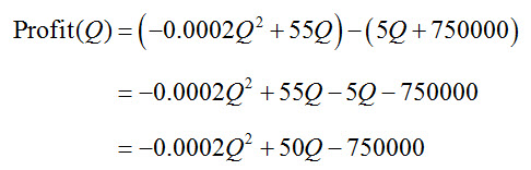
The cost of producing robotic hamsters at an Asian manufacturing plant is
Cost(Q) = 5Q + 750000 dollars
where Q is the number of robotic hamsters. The revenue from selling the toys is
Revenue(Q) = -0.0002Q2 + 55Q dollars.
a. Find the profit function.
Solution The profit function is formed by subtracting Cost(Q) from Revenue(Q),
This function is a quadratic function of Q with a = -0.0002, b = 50, and c = -750000.
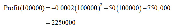
b. Find the profit at a production level of 100,000 robotic hamsters.
Solution Substitute Q equal to 100,000 into the profit function, Profit(Q) = -0.0002Q2 + 50Q -750,000, to yield
At a production level of 100,000 robotic hamsters, the profit is $2,250,000.
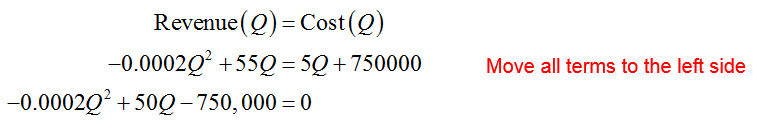
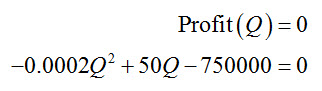
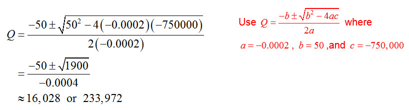
c. Find the break-even quantity.
Solution We have two options for finding the break-even quantity. Set the revenue equal to the cost function and solve for Q or set the profit function equal to zero. If we set the revenue equal to the cost,
Notice that moving all terms to the left side is the same as setting the profit function equal to zero,
We could try to factor this quadratic equation to solve it, but it is easier to use the quadratic formula:
Each quantity occurs at a decimal value. To insure we have at least broken even, round each quantity to the nearest integer so that profit is slightly positive.
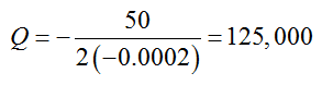
d. Does the profit function have a high point or low point? Where is this point?
Solution For this parabola, a < 0. This mean the graph has a high point. Since the independent variable in this problem is Q, the high point is located using the formula.
This gives us a production level of
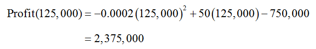
To locate this point, we also need to find the profit at the break-even quantity. Putting this production level into the profit function yields
In later chapters we’ll learn how to find the high and low points on any function using calculus. Finding these points is one of the useful applications for calculus.
How do you calculate the average rate of change from a table?
We quantify how one quantity changes with respect to another using the average rate of change.
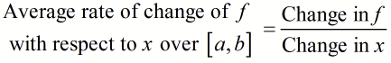
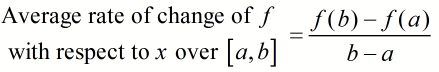
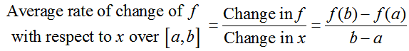
Average Rate of Change The average rate of change of f with respect to x from x = a to x = b is defined as
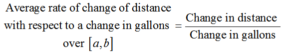
Since the numerator and denominator each contain a difference of two values, the quotient or the right side of the definition is often called a difference quotient. The variable x describes one of the quantities we are interested in comparing and the variable f describes the other quantity. In general, one of the quantities is thought to depend on the other. The quantity that depends on the other corresponds to the dependent variable f and the variable x, the independent variable, corresponds to the other. Often the choice of which quantity is which is not very clear cut. In many of those cases, we can use the units on the comparison to determine how the average rate of change should be computed. For instance, suppose the auto manufacturer is interested in the miles per gallon that its vehicles achieve. This means they wish to calculate how the miles change with respect to the change in the gallons in the tank. In this case, they would think of this average rate of change as The numerator of this difference quotient is in miles and the denominator is in gallons yielding units of miles per gallon on the average rate of change. In this case, we would think of the distance traveled as being dependent on the number of gallons in the tank of the automobile. A general guideline to use is when we discuss the average rate of change of quantity f with respect to a quantity x, the change in the quantity f is in the numerator of the difference quotient. The change in the quantity x is in the denominator of the difference quotient. The average rate of change can be a positive number or a negative number. If the average rate of change is a positive number, the quantity corresponding to the numerator of the difference quotient increases as the quantity in the denominator increases. On the other hand, if the quantity in the numerator decreases as the quantity in the denominator increases, then the average rate of change is negative. The average rate of change can be viewed in many different ways. To make it as simple as possible, it is useful to work with the definition in all situations, and then adapt this definition to specific applications. Keep in mind that the numerator and denominator each describe changes in some quantities. The units on the average rate of change correspond to the units on the quantities in the numerator and denominator.
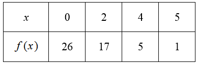
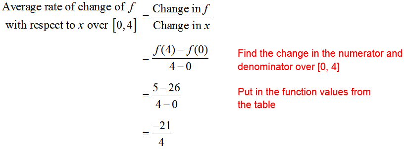
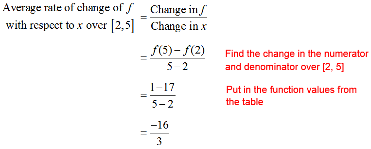
Example 1 Find the Average Rate of Change from a Table
The table below defines the relationship y = f (x). Use this table to compute the average rates of change below.
a. Find the average rate of change of f with respect to x over [0, 4].
Solution Apply the definition of the average rate of change to give b. Find the average rate of change of from x = 2 to x = 5.
Solution In this part, the interval is defined with slightly different phrasing. By saying, “from x = 2 to x = 5”, the interval over which the average rate of change is being found is being defined to be [2, 5]. Using the definition for average rate of change yields Note that what you are doing is calculating the slope between the ordered pairs (2, 5) and (5, 26). In both parts, the average rate of change is negative indicating that f (x) decreases as x increases.
Example 2 Find the Average Rate of Change from a Table
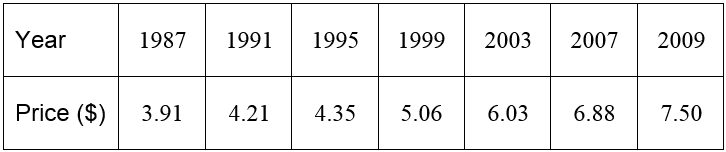
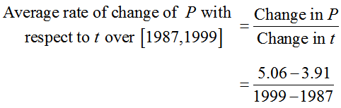
The average price for a ticket to a movie theater in North America for selected years is shown in the table below. (Source: National Association of Theater Owners, www.natoonline.org) In each part, calculate the indicated average rate of change.
a. Find the average rate of change of ticket price with respect to time over the period 1987 to 1999.
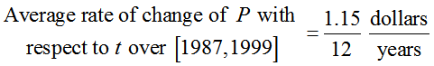
Solution Use the definition of average rate of change to write as From the table we know the price of a ticket in 1987 was $3.91 and the price of a ticket in 1999 was $5.06. The average rate of change of P with respect to t from t = 1987 to t = 1999 is The numerator of this quotient is a difference in prices and corresponds to a change of 1.15 dollars. The denominator is a difference in years and corresponds to a change of 12 years. The difference quotient is If we round this average rate of change to the nearest cent, we get approximately 0.10 dollars per year. This tells us that each year from 1987 through 1999, the ticket prices rose by an average of about 0.10 dollars or 10 cents.
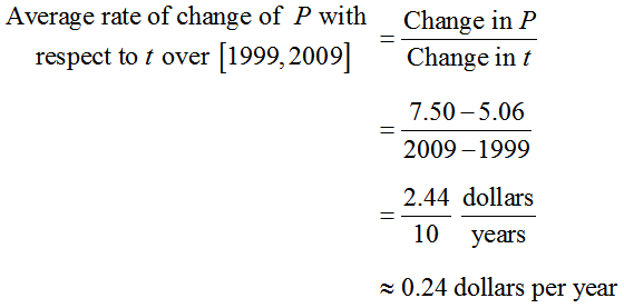
b. Find the average rate of change of ticket price with respect to time over the period 1999 to 2009.
Solution The price of a ticket in 1999 was $5.06 and $7.50 in 2009. The averate rate of change of P with respect to t from t = 1999 to t = 2009 is This means that ticket prices increased by an average of approximately 0.24 dollars or 24 cents each year from 1999 to 2009.
c. Were ticket prices increasing faster during the period from 1987 to 1999 or during the period 1999 to 2009?
Solution The time period with the greater average rate of change corresponds to the period in which the prices are increasing faster. Since the average rate of change of price from 1999 to 2009 is approximately 0.24 dollars per year and the average rate of change of price from 1987 to 1999 is approximately 0.10 dollars, prices are rising faster from 1999 to 2009.
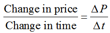
The numerator and denominator of the difference quotient is often symbolized using the greek symbol capital delta, ∆. For the average rate of change of price with respect to time, we could symbolize the difference quotient as where we think of the symbol ∆ as indicating “change in”. The symbol ∆P corresponds to a change in price since P represents price. This symbol helps us to economize on the amount of writing we need to do in order to indicate an average rate of change. In Example 1 and Example 2, there were only two rows of data in the table. It was fairly easy to decide what numbers go in the numerator of the difference quotient and which numbers go in the denominator of the difference quotient. In the next example, there are several columns of data and we’ll need to examine the average rate of change to determine how the difference quotient is formed.
Example 3 Find the Average Rate of Change from a Table
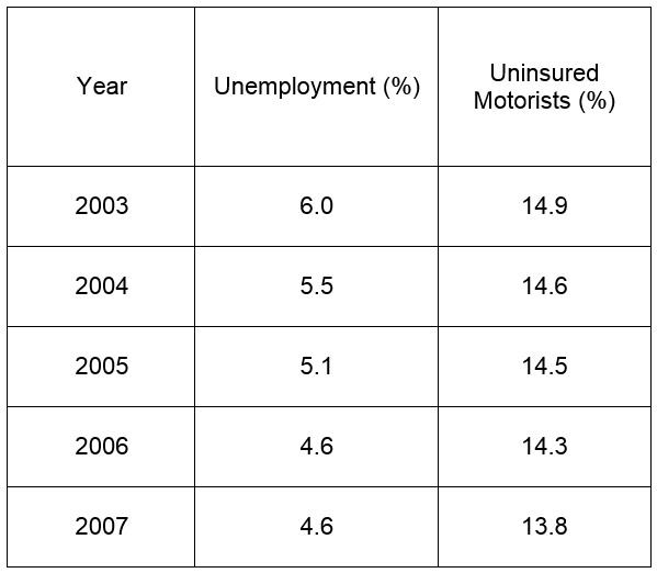
During the years 2003 through 2007, the percentage of Americans unemployed and the percentage of Americans driving without auto insurance both dropped according to the table below: (Source: Insurance Research Council)
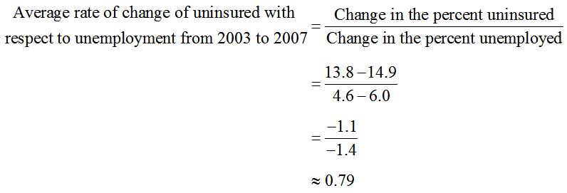
a. Find the average rate of change of uninsured with respect to unemployment over the period 2003 through 2007.
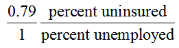
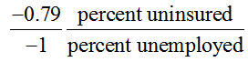
Solution We are interested in how the percent uninsured changes as the percent uninsured changes. The time period is not a part of the average rate of change except to reference the values for the percent unemployed and the percent of motorists that are unemployed. We could think of the values in the table as function values, however in this case we’ll simply think of the average rate as a ratio of changes. The average rate of change of the percent uninsured with respect to the percent unemployed is computed as The years serve to reference the particular data we’ll use to compute the change, but are not otherwise involved in the calculation. Using the percent uninsured and unemployed in 2003 (6% unemployed and 14.9% uninsured) and 2007 (4.6% unemployed and 13.8 uninsured), we get The unit on the numerator of the difference quotient is percent uninsured and the unit on the denominator of the difference quotient is percent unemployed. This means the units on the average rate of change is percent uninsured per percent unemployed.
b. In a new release, an official with the Insurance Research Council was quoted as saying, “”If the unemployment rate goes up by 1 percent, we would anticipate that the percentage of people who are uninsured would go up by three-fourths of 1 percent.” Use the data from in 2003 and 2007 to support this statement.
Solution In part a, we calculated the average rate of change of the percent uninsured with respect to the percent unemployed as 0.79 over this time period. The units on this number are percent uninsured per percent unemployed. Think of the average rate as Then the rate can be interpreted as a 1 percent change in unemployment leads to a 0.79 percent change in the percent of motorists that are uninsured. Although this is not exactly a change of “three-fourths of 1 percent”, it is close enough to be consistent. In popular media, a phrase like “three-fourths of 1 percent” is more palatable than the number 0.79 percent. It is interesting to note that even though the percents are both decreasing, the average rate of change is interpreted in terms of increases. We could have also interpreted the average rate as In this case we would say that a 1 percent drop in the percent unemployed leads to a 0.79 percent drop in the percent of motorists uninsured.
How do you calculate the average rate of change from a function?
When a function is given by a formula, we modify the definition of average rate of change:
Average Rate of Change
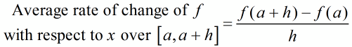
The average rate of change of f (x) with respect to x from x = a to x = b is defined as
Close examination of this definition reveals that it is simply the same definition as before, but with
so that we can write
Instead of using the data values to calculate the changes in the difference quotient, we use the function’s formula to get the values in the numerator of the difference quotient.
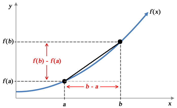
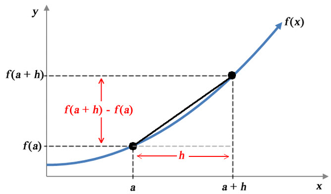
In the context of the graph of a function, the average rate of change of a function can be visualized as the slope of a line that passes through two points on the function. This line, called a secant line, can be drawn on a graph of a function so that we can quantify the value of the slope of the line.
Figure 1 – The average rate of change of f (x) with respect to x over [a, b] is equal to the slope of a line of a secant line.
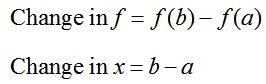
A secant line passing through the points (a, f (a)) and (b, f (b)) has a vertical rise of f (b) – f (a) and a horizontal run of b – a. The slope of between the points on the secant line is
Example 4 Find the Average Rate of Change from a Function’s Formula
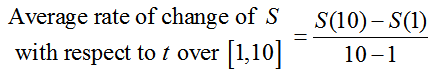
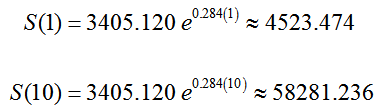
The annual sales (in millions of dollars) at Apple from 2001 through 2010 can be modeled by
where t is the number of years since 2000. Find the average rate of change of sales with respect to time over the period from 2001 to 2010.
(Modeled from Apple Annual Reports)
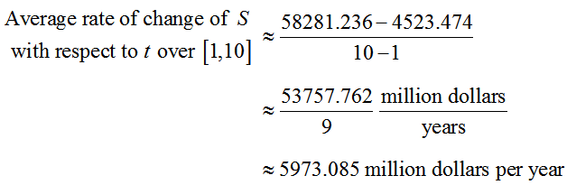
Solution Using the definition of the average rate of change,
The function values in the numerator are computed from the function’s formula,
This leads to the average rate of change,
Each decimal is written to three decimal places since the decimals in the original function were written to three decimal places. This average rate tells us that the sales increased by an average of about 5973.085 million dollars or $5,973,085,000 in each year from 2001 through 2010.
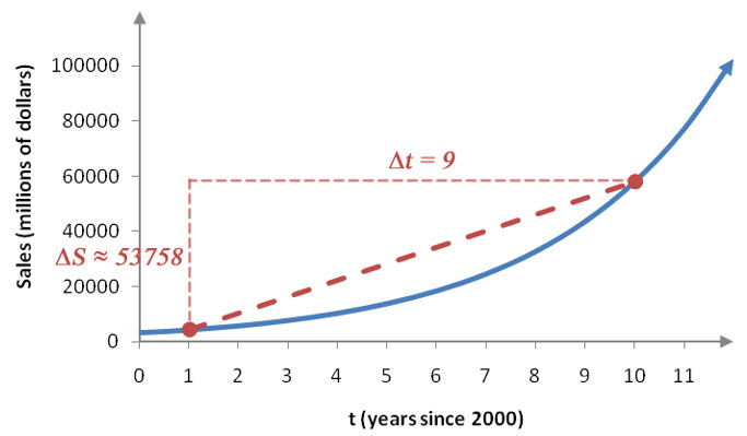
On a graph of the sales function S(t), the average rate of change of sales from t = 1 to t = 10 may be visualized as the slope of the line connecting the points at (1, S(1)) and (10, S(10)).
Figure 2 – The slope of the line connecting the sales at t = 1 and t = 10 is the same as the average rate of change between these points.
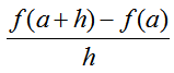
In calculus, one difference quotient in particular comes up very often.
The average rate of change of f (x) with respect to x from x = a to x = a + h is
This is the same definition we have been using with functions given by formulas, but with b = a + h. The value of h is the horizontal separation of the two points on the secant line. This difference quotient will be very important in defining the instantaneous rate of change in Section 11.2.
Example 5 Find the Difference Quotient
Let f (x)be defined by
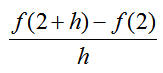
a. Find and simplify the difference quotient
Solution This difference quotient is
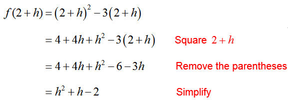
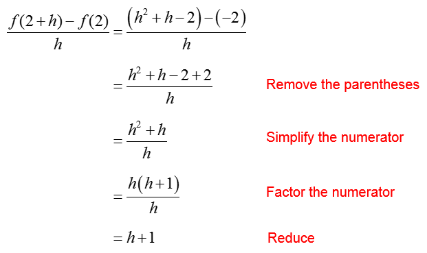
with a = 2. Find the function values in the numerator of the difference quotient. The value f (2)is found by replacing x with 2 in the function,
Similarly, f (2 + h) is found by replacing x with 2 + h,
Substitute these function values into the difference quotient to yield
b. Evaluate the difference quotient in part a when h = 0.25.
Solution The expression for the difference quotient in part a, h + 1, makes it easy to evaluate the difference quotient for any value of h. It enables us to find the average rate of change of f (x) with respect to x from x = 2 and any other x value.
Set h = 0.25 to give
This value is the average rate of change of f (x) with respect to x from x = 2 to x = 2 + 0.25.
Care must be taken to calculate f (a + h) in the difference quotient. The most common mistake in simplifying the function value f (a + h) is to assume it is the sum of the values of the function. For instance, in the previous example f (2 + h) ≠ f (2) + f (h). The powers on the factors correspond to multiplication. They must be worked out when calculating f (a + h).
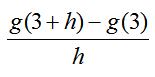
Example 6 Find the Difference Quotient
Find and simplify the difference quotient
for the function
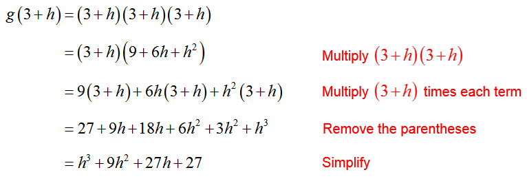
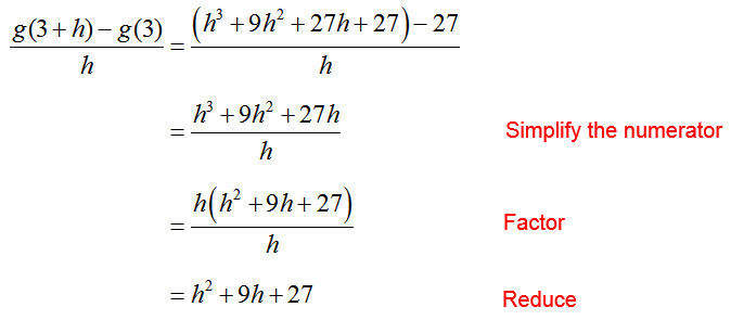
Solution To find the difference quotient, we must evaluate g(t) at 3 and 3 + h. The value g(3) = 33 = 27 is easy to calculate. However g(3 + h) is more challenging:
To simplify the expression on the right, we need to cube the quantity 3 + h,
Now we can put the function values into the difference quotient and simplify: