Category: Applied Calculus Ebook

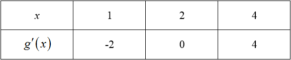
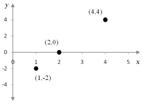
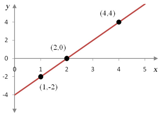
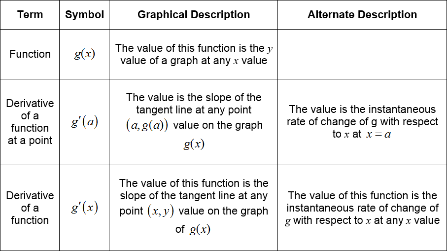
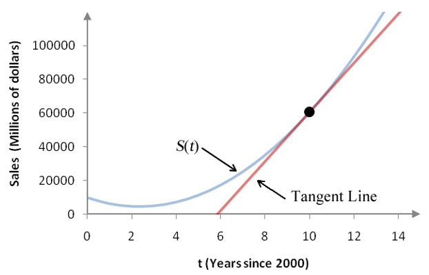
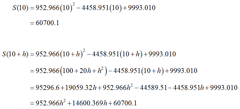
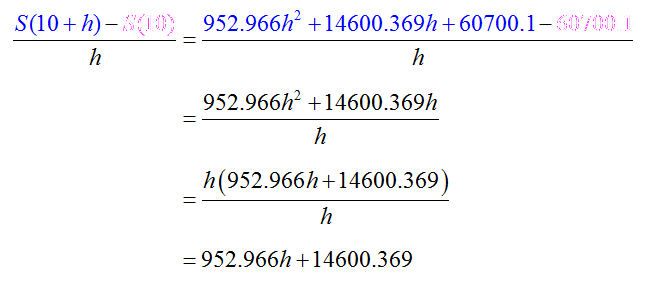
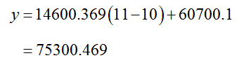
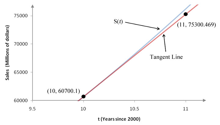
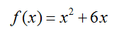
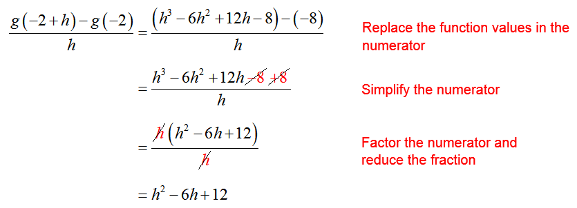
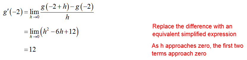
How do you calculate the derivative of a function from the definition?

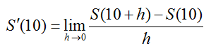
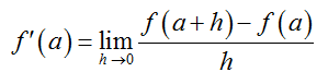
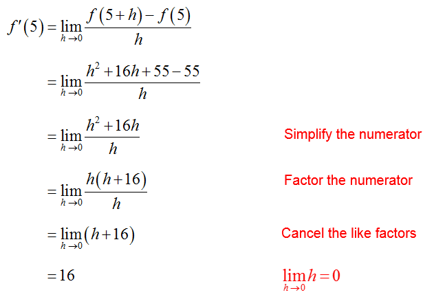
The definition of the derivative of a function f (x) at a point x = a was given in Section 11.3,

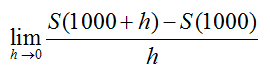
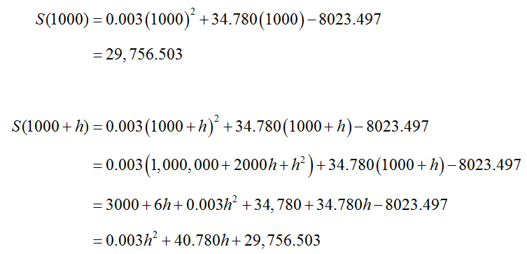
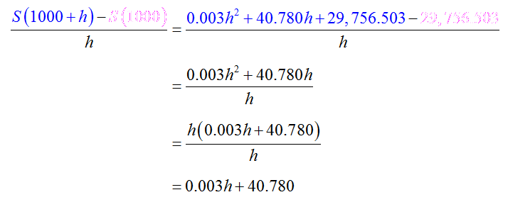
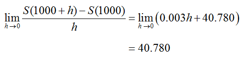
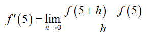
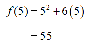
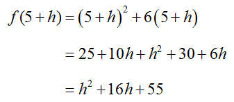
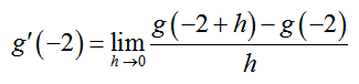
$$f’\left( a \right) = \mathop {\lim }\limits_{h\,\, \to 0} \frac{{f(a + h) – f(a)}}{h}$$

provided this limit exists. We can adapt this definition to find the derivative of a function by changing the constant a to a variable x.

We can apply this definition in a manner similar to how we applied the definition of derivative of a function at a point.

Let’s use this strategy to find the derivatives of several functions.

Example 2        Find the Derivative

Use the definition of the derivative to find the derivative of the function $$f(x) = 2x – 7$$

Solution To apply the definition of the derivative to this function, we must evaluate f (x + h). Replace x in the function with x + h  to yield $$\displaylines{
f(x + h) = 2\left( {x + h} \right) – 7 \cr
= 2x + 2h – 7 \cr} $$

It is important to note that we are replacing x with the group  x + h in parentheses. Now form the difference quotient,$$\frac{{f(x + h) – f(x)}}{h} = \frac{{\left( {2x + 2h – 7} \right) – \left( {2x – 7} \right)}}{h}$$

To make the limit easy to evaluate, let’s simplify the difference quotient as much as possible.

$$
\begin{align*}
\frac{{f(x + h) – f(x)}}{h} &= \frac{{\left( {2x + 2h – 7} \right) – \left( {2x – 7} \right)}}{h} && {\color{red}{\small \text{Remove the parentheses and subtract each term}}} \cr
&= \frac{{2x + 2h – 7 \color{red}{- 2x + 7}}}{h} && \cr
&= \frac{{2 \color{red}{h}}}{\color{red}{h}} && {\color{red}{\small \text{Combine like terms}}} \cr
&= 2 && {\color{red}{\small \text{Reduce the quotient}}} \cr
\end{align*} $$

Substitute this expression into the definition of the derivative:

$$\begin{align*}
f'(x) &= \mathop {\lim }\limits_{h\,\, \to 0} \frac{{f(x + h) – f(x)}}{h} \cr
&= \mathop {\lim }\limits_{h\,\, \to 0} 2 \cr
&= 2 \cr \end{align*}$$
The derivative of the linear function $f(x) = 2x – 7$ is $f'(x) = 2$.

Example 3        Find the Derivative

Use the definition of the derivative to find the derivative of the function$$g(t) = {t^2} + 3t + 7$$

Solution In this example, we’ll follow the same strategy for finding the derivative. However, since the name of the function is g(t), we need to adjust the definition of the derivative to read$$g'(t) = \mathop {\lim }\limits_{h\,\, \to 0} \frac{{g(t + h) – g(t)}}{h}$$

Substitute t + h  for t in g(t) to give
$$
\begin{align*}
g(t + h) &= {\left( {t + h} \right)^2} + 3\left( {t + h} \right) + 7 && \cr
&= {t^2} + 2ht + {h^{^2}} + 3\left( {t + h} \right) + 7 && \color{red}{\small \text{Multiply }} \color{red}{\left( {t+h} \right)\left( {t+h} \right)} \cr
&= {t^2} + 2ht + {h^2} + 3t + 3h + 7 && \color{red}{\small \text{Multiply 3 times }} \color{red}{t+h} \cr
\end{align*}
$$

If we place this expression and the expression for  into the numerator of the difference quotient, we get

$$\begin{align*}
\frac{{g(t + h) – g(t)}}{h} &= \frac{{\left( {{t^2} + 2ht + {h^2} + 3t + 3h + 7} \right) – \left( {{t^2} + 3t + 7} \right)}}{h} && \color{red}{\small \text{Subtract and simplify}} \cr
&= \frac{{{t^2} + 2ht + {h^2} + 3t + 3h + 7 \color{red}{- {t^2} – 3t – 7}}}{h} && \color{red}{\small \text{Combine like terms}} \cr
&= \frac{{2ht + {h^2} + 3h}}{h} && \cr
&= \frac{{\color{red}{h}\left( {2t + h + 3} \right)}}{\color{red}{h}} && \color{red}{{\small \text{Factor }}h{\text{ and reduce}}} \cr
&= 2t + h + 3 && \cr
\end{align*}
$$

With this expression in the definition of the derivative, we write
$$
\begin{align*}
g'(t) &= \mathop {\lim }\limits_{h\,\, \to 0} \frac{{g(t + h) – g(t)}}{h} \cr
&= \mathop {\lim }\limits_{h\,\, \to 0} \left( {2t + h + 3} \right) \cr
&= 2t + 3 \cr
\end{align*}
$$

The derivative of the quadratic function $g(t) = {t^2} + 3t + 7$ is the linear function $g'(t) = 2t + 3$.

Example 4        Find the Derivative

Use the definition of the derivative to find the derivative of the function$$j(t) = {e^t}$$

Solution The definition of the derivative for this function is$$j'(t) = \mathop {\lim }\limits_{h\,\, \to 0} \frac{{j(t + h) – j(t)}}{h}$$

Using the exponential function, the difference quotient is$$\frac{{j(t + h) – j(t)}}{h} = \frac{{{e^{t + h}} – {e^t}}}{h}$$

This expression can be simplified, but not as easily as Example 2 or Example 3.

In this case we rewrite ${e^{t + h}}$ as ${e^t}\;{e^h}$. By doing this, we can factor the numerator:

$$
\begin{align*}
\frac{{j(t + h) – j(t)}}{h} &= \frac{{{e^{t + h}} – {e^t}}}{h} \cr
&= \frac{{{e^t}\;{e^h} – {e^t}}}{h} \cr
&= \frac{{{e^t}\left( {{e^h} – 1} \right)}}{h} \cr
\end{align*}
$$

From this simplified difference quotient, we can write out the definition of the derivative,
$$
\begin{align*}
j'(t) &= \mathop {\lim }\limits_{h\,\, \to 0} \frac{{j(t + h) – j(t)}}{h} \cr
&= \mathop {\lim }\limits_{h\,\, \to 0} \frac{{{e^t}\left( {{e^h} – 1} \right)}}{h} \cr
&= {e^t} \cdot \mathop {\lim }\limits_{h\,\, \to 0} \frac{{{e^h} – 1}}{h} \cr
\end{align*}
$$

The factor ${e^t}$ is a constant with respect to h, so it can be moved outside the limit. To complete the derivative, we must evaluate the limit.

For this limit we’ll find the limit by creating a table of values for  for smaller and smaller h values.

The table suggests that as x gets smaller and smaller, the value of the quotient approaches 1 or $$\mathop {\lim }\limits_{h\,\, \to 0} \frac{{{e^h} – 1}}{h} = 1$$

Using $\mathop {\lim }\limits_{h\,\, \to 0} \frac{{{e^h} – 1}}{h} = 1$ in the expression for the definition of the derivative yields

$$
\begin{align*}
j'(t) &= {e^t} \cdot \mathop {\lim }\limits_{h\,\, \to 0} \frac{{{e^h} – 1}}{h} \cr
&= {e^t} \cdot 1 \cr
&= {e^t} \cr
\end{align*}
$$

The derivative of $j(t) = {e^t}$  is $j'(t) = {e^t}$.

What is a derivative function?

Let’s examine the tangent line on the function pictured in Figure 1.

Figure 1 – A quadratic function g(x) (blue) with a tangent line (red) at x = 1.

We can approximate the value of the derivative at x = 1 or g′(1) by calculating the slope of the tangent line at x = 1. Any two points on the tangent line can be used to make an estimate of the slope.

Figure 2 – The points (0, 4) and (2, 0) can be used to estimate the slope of the tangent line at x = 1.

From Figure 2, we see that the slope of the tangent line or g′(1) is approximately ^-4/₂ or -2. Any other two points on the line could be used to calculate this slope. For instance, the points (1, 2) and (2, 0) are on the tangent line. The slope between these points is
$$ g’\left( 1 \right) \approx \frac{{2 – 0}}{{1 – 2}} = – 2 $$

Different points don’t always lead to exactly the same slope, but they should be close. If we look at the tangent line for g(x) at x = 2, we see that it is horizontal and passes through the point (2, 1).

Figure 3 – The tangent line to g(x) at x = 2 is a horizontal tangent line.

Since the tangent line is horizontal, its slope is zero. This tells us that g′(2) = 0.

Let’s estimate the slope of one more tangent line at x = 4.

Figure 4 – The tangent line to g(x) at x = 4 passes through the points (3,1) and (5,9).

The slope is calculated as
$$g’\left( 4 \right) \approx \frac{{9 – 1}}{{5 – 3}} = \frac{8}{2} = 4$$

With these three tangent lines, we can organize the slopes in a table.

If we graph these values with the x values as the independent variable and the slopes as the dependent variable, we see a pattern emerge.

Figure 5 – In this graph, the slopes of the quadratic function are graphed at corresponding x values.

The slopes appear to lie along a straight line. If we draw this line through the points we can use it to find the slope of the tangent line at other x values.

Figure 6 – Each of the slopes of the quadratic function lie along a straight line.

For instance, at x = 3 the line passes though y = 2 . This means the slope of the tangent line at x = 3 on the quadratic function is 2. The function corresponding to this line is called the derivative of the quadratic function g(x) and is denoted by g′(x).

All of these concepts can be a bit confusing. So let’s recap these different ideas using a function g(x). Keep in mind that we could use any name in place of g and any variable in place of x.

Example 1    Find the Derivative Function

The graph of the function f (x) is shown below.

Find the graph of the derivative function f ′(x) using the tangent lines to the function f (x).

Solution To find the derivative of the function, we’ll draw tangent lines along the function, record the slopes in a table and graph the corresponding ordered pairs.

Using the grid on the graph, we see that the tangent line passes through (-3, 0) and (-2, 1.8). The slope of the tangent line is approximately
$$f'( – 3) = \frac{{1.8 – 0}}{{ – 2 – ( – 3)}} = 1.8$$

We’ll continue to fill out the table of tangent line slopes:

Our ability to calculate the slope is constrained by our ability to locate points on the tangent line. For this tangent line, the points (-2, 1) and (1, 1.9) are on the line. The slope of the tangent line is approximately
$$f'( – 2) = \frac{{1.9 – 1}}{{1 – ( – 2)}} = 0.3$$

At the next row in the table, we find the slope of the tangent line at x = -1:

Any two points on the tangent line can be used to find the slope. For this tangent line, the points (-3, 2) and (2, -1) are on the line. The slope of the tangent line is approximately

$$f'( – 1) = \frac{{ – 1 – 2}}{{2 – ( – 3)}} = – 0.6$$

If we continue to find the slopes of tangent lines at each of the x values in the table, we can graph the ordered pairs in the form (x, f ′(x)). This means that we graph the x values horizontally and the f ′(x) values vertically.

These ordered pairs lie on the derivative function f ′(x).

If we were to graph more points on the derivative function, we would see a graph like the one below.

Usually it is not necessary to graph a large number of points to graph the derivative function. Typically a few points on the graph are enough to display the overall pattern. Then the rest of the graph can be sketched to approximate the pattern.

What does the derivative at a point tell you about a function?

The derivative at a point is a rate so we may interpret it like any other rate of change. In general, we can use the units on the independent and dependent variable to find the units on the derivative.

Suppose a function is given by y = f (x) where x is the independent variable and y is the dependent variable. The units on the derivative of f (x) at x = a are

Once we have established the units on the derivative, we can use them to interpret what the derivative means.

Example 5    Find and Interpret the Derivative

Based on data from 2001 through 2010, the annual sales at Apple (in millions of dollars) can be modeled by

where R is the amount spent annually on research and development in millions of dollars.

a.   Find S′(1000).

Solution Using the definition of the derivative at a point, we must compute

We’ll do this by computing S(1000) and S(1000 + h). From these values and expressions we’ll form the difference quotient , simplify, and evaluate the limit.

Let’s look at the terms in the numerator of the difference quotient:

Now form the difference quotient and simplify:

The limit as h approaches 0 yields

The derivative is S′(1000) = 40.780.

b. What does the value you calculated in part a tell you about the relationship between sales and money spent on research and development?

Solution To interpret the derivative in part a, we need to establish the units on the derivative. A derivative has the same units as an average rate of change or an instantaneous rate of change for the function S(R),

In the case of the derivative S′(R), the units are

Notice that the numerator and denominator both are in millions of dollars. To distinguish the dollars of sales from the dollars of research and development, labels indicating the origin of the money are included.

The factor of millions in the numerator and denominator may be divided out to yield

The statement S′(1000) = 40.780 means that at a level of 1000 million dollars of research and development, sales are increasing at a rate of 40.78 dollars of sales per dollar of research and development. In other words, if research and development is increased by 1 dollar at this point, sales will increase by approximately 40.78 dollars.

How can you use a tangent line to forecast function values?

Tangent lines can be used to estimate values for functions. These estimations, called straight line or linear approximations, are often used to predict model values beyond the range of data used to create the model. For instance, the function S(t) graphed in Figure 11 models sales at Apple Inc. from 2001 through 2010. This means the data used to create the function range from t = 1 through t = 10 . This region of the graph is shaded yellow.

Figure 11 – A graph of the sales S(t) as a function of the number of years t based on sales data from 2001 through 2010.

If we use the model to determine the sales in the shaded region, we are interpolating the sales. Interpolation is the process of finding values for the model in the range of the data used to create the model.

We are interested in extrapolating the sales. Extrapolation is the process of finding values for the model outside the range of data values used to create the model. We want to use this model to extrapolate the sales in 2011.

We have two options for finding the sales. We could use the function to calculate the sales. Alternately, we could use the tangent line to S(t) at t = 10 to find the sales.

Figure 12 – The model S(t) with the tangent line to S(t) at t = 10.

In Figure 13, we see that the model S(t) and the tangent line are identical at t = 10. To the right of t = 10, the slope of the model S(t) increases so the graph curves upward. Over the same values, the tangent line increases at a constant rate equal to the derivative of S(t) at t = 10 or S′(10). Because of the differences in how the two graphs behave, the model and the tangent line slowly separate.

Figure 13 – S(t) and the tangent line to S(t) at t = 10 in the small interval [10, 11].

As we move even farther beyond the shaded region, the gap between the two functions becomes larger. The model S(t) increases faster and faster meaning sales must be increasing faster and faster. The tangent line increases at a constant rate of S′(t). Either graph can be used to predict the sales after t = 10, but under different assumptions.

Figure 14 – A bigger picture of the model S(t), its tangent line at t = 10, and the region where the data used to find the model are located.

If we use the function S(t) to predict the sales in 2011 and find S(11), then we are assuming that rate that sales are changing will increase. Some might call this an optimistic prediction.

If we use the tangent line to predict the sales in 2011, we are assuming that sales will grow at a constant rate. This rate is the same as the rate the sales were changing in 2010. Since sales are not growing as fast in this prediction, we might think of this estimate as being more conservative. This estimate is smaller than the estimate .

Example 4    Forecast Sales Using a Tangent Line

The sales S(t) at Apple Computer from 2001 to 2010 are given by the function

where t is the number of years after 2000. Assume this model is valid for values of t in the interval [1, 10].

a. Use the tangent line at t = 10 to forecast the sales in 2011.

Solution To find the tangent line at t = 10, we must first calculate the value of S′(10). In this context, the definition of the derivative at a point is

Start by computing the function values:

These values must be substituted into the definition for S′(10).

As with previous examples, simplifying the numerator allows the difference quotient to be simplified:

To find the value of the derivative, we must evaluate the limit,

As h approaches zero, the first term in the limit approaches zero and the second term is independent of h. This means that S′(10) = 14600.369. This value is the slope of the tangent line.

The equation of the tangent line can be written using the point-slope form of a line y – y₀ = m(t – t₀) where m is the slope of the tangent line. The point (t₀, y₀) is the point on S(t) that the tangent line passes through.

The tangent line is to pass through t = 10. To find the derivative, we calculated S(10) = 60700.1 and now we can use this value to give the equation of the tangent line,

Solve this equation for y to yield

To forecast the sales in 2011, we substitute t = 11 into the equation for the tangent line,

Following the tangent line, the sales at Apple Computer in 2011 will be 75300.469 million dollars or $75,300,469,000.

Figure 15 – The sales function S(t) is quadratic and curves upward. The tangent line uses the instantaneous rate of change at t = 10 and projects sales into the future. Since the tangent line does not curve, the projection falls farther and farther from the sales function S(t) the farther we project from t = 10.

 b. How does the linear approximation in 2011 compare the model’s prediction in 2011?

Solution The model’s prediction in 2011 is

From part a, we know the linear approximation is 75,300.469 million dollars. Since the model is curving upward, its estimate is higher than the linear approximation by 76,253.435 – 75,300.469 or 952.966 million dollars. This difference may not seem like much, but is almost 1 billion dollars.

Figure 16 – The estimates of sales in 2011 based on the model S(t) and the tangent line to  S(t) at t = 10.

On the tangent line in Example 4 each unit we move to the right horizontally corresponds to a vertical increase of 14600.369. Thus a simple way to view the estimate at t = 11 is to take the sales at t = 10 and add 14600.369,

60700.1 + 14600.369 = 75300.469

We can expand on this reasoning to make estimates of the sales at other points along the tangent line:

In each case, we multiply the slope by the number of units from t = 10 and add the product to or 60700.1.

Figure 17 – The linear approximation can be visualized with the slope of the tangent line labeled carefully.

In Figure 17, we see that for each year after t = 10 the tangent line rises by 14600.369 million dollars. This is why we can approximate values along the tangent line by adding the sales at t = 10 to the product of the number of years from t = 10 times the slope of the tangent line.

How do you compute the derivative at a point using a limit?

In the previous question, we estimated the value of the derivative by estimating the slope of the tangent line on the graph of the function. If the function is given by a formula, we can find an exact value for the derivative at a point by applying the definition of the derivative directly. Recall that the derivative of a function y = f (x) at the point (a, f (a)) is defined by the limit

provided this limit exists. For many functions, we can find the value of the derivative by following several steps that help us to systematically evaluate the limit.

We’ll use this strategy to find the derivatives of several different functions evaluated at a point.

 Example 2    Compute the Derivative at a Point Using a Limit

Suppose the function f (x) is given by

Use the definition of the derivative at a point to compute f ′(5).

Solution The value of f ′(5) is found by evaluating the limit

The function values in the numerator are

and

Using these values in the definition of the derivative yields

The value of the derivative of f (x) at x = 5, f ′(5), is 16.

Example 3    Compute the Derivative at a Point Using a Limit

Suppose the function g (t) is given by

Use the definition of the derivative at a point to compute g′(-2).

Solution This function is named g(t) instead of f (x), so we need to modify the definition of the derivative of f (x) at a point x = a. Using g(t) in the definition and the point t = -2, we have

The function value g(-2) is calculated to be

The function value g(-2 + h) must be calculated carefully.

Form the difference quotient and simplify:

The derivative is completed by taking the limit as h approaches zero,

The derivative of g(t) evaluated at t = -2, g′(-2), is 12.