Category: Applied Calculus Ebook

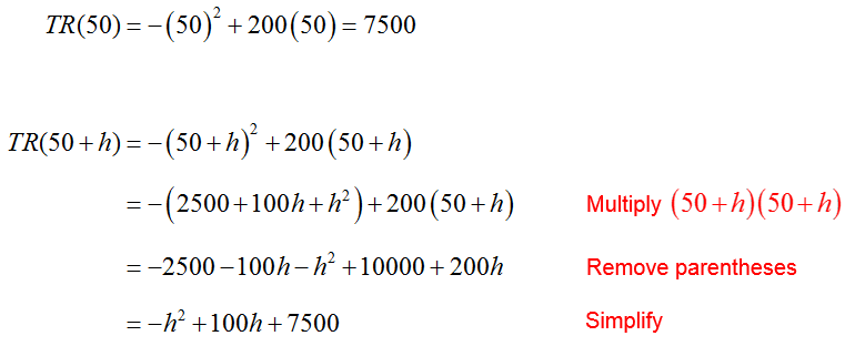
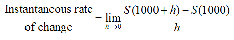
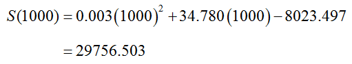
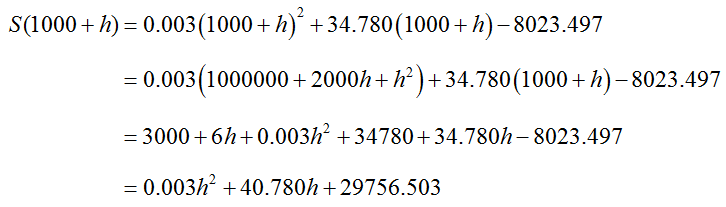
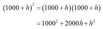
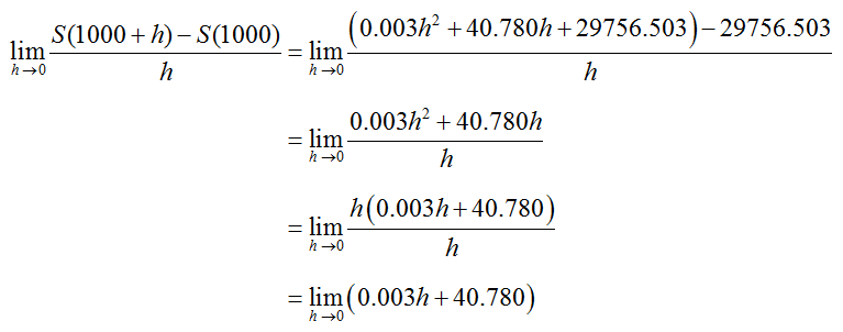
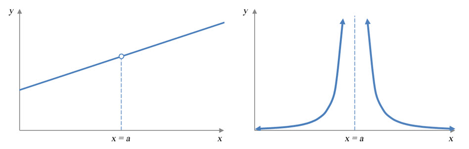
What is a derivative?

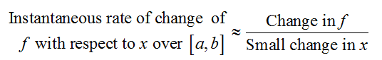
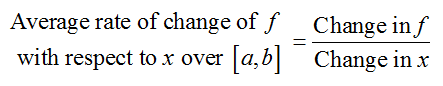
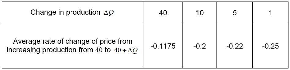
The derivative of a function at a point is closely related to the average rate of change of a function. To understand this relationship geometrically, let’s look at average rate of change of a function in the context of the slope of a secant line. We’ll use the graph below to illustrate this relationship. This graph shows the weighted average price per bushel for oats in dollars as a function of the annual production of oats in the United States in millions of bushels.

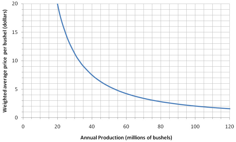
Figure 1 – The demand function describing the relationship between the annual production of oats and the weighted average price of oats.

This function decreases since the price drops as the annual production increases. This behavior is typical of demand functions.

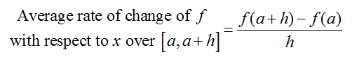
The average rate of change of the price per bushel with respect to annual production is found by calculating the change in the weighted average price per bushel, ΔP, and dividing that value by the change in the annual production, ΔQ. The average rate of change of weighted average price from an annual production level of 40 million bushels to 80 million bushels is

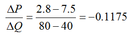
Since the numerator has units of dollars and the denominator has units of millions of bushels, the units on the average rate of change are of dollars per million bushels. The average rate of change is the same as the slope of the secant line, so the slope of the secant line in Figure 1 is -0.1175.

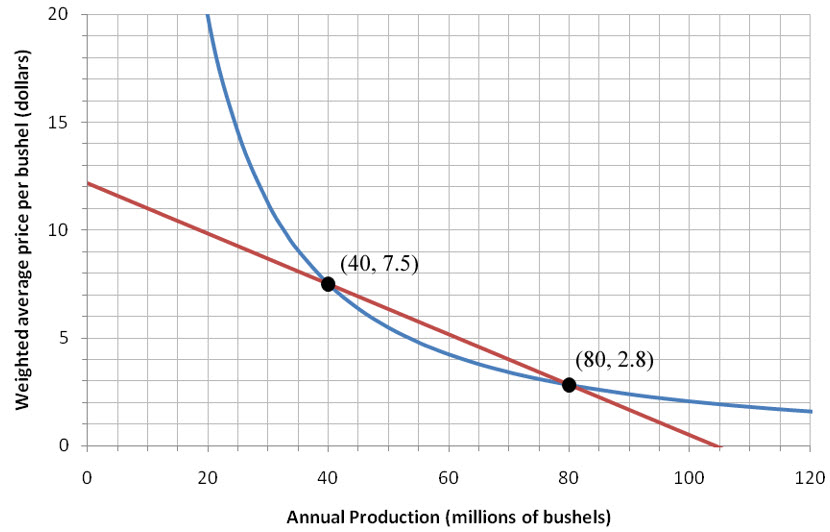
Figure 2 – The demand function for oat production (blue) with a secant line (red) passing through the production levels of 40 and 80 million bushels.

We are interested in approximating the instantaneous rate of change of the price with respect to the annual production at an annual production level of 40 million bushels. To do this, we need to find the average rate of change of the price over smaller and smaller changes in production near an annual production level of 40 million bushels. If we calculate the average rate of change between 40 and 50 million bushels instead of 40 and 80 million bushels, we obtain

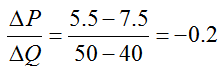
This average rate of change is identical to the slope of the secant line passing through (40, 7.5) and (50, 5.5) pictured in Figure 2.

Figure 3 – The demand function for oat production (blue) with a secant line (red) passing through the production levels of 40 and 50 million bushels.

We can continue to find the average rate of change in price with respect to the change in annual production for smaller and smaller intervals. The average rate of change of price with respect to a change in annual production from 40 million bushels to 45 million bushels is

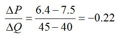
The slope of the secant line passing through (40, 7.5) and (45, 6.4) is also -0.22. This secant line is graphed with the demand function in Figure 3.

Figure 4 – The demand function for oat production (blue) with a secant line (red) passing through the production levels of 40 and 45 million bushels.

As we calculated the average rate of change of prices with respect to annual production for smaller and smaller changes in annual production, the values became more negative. If we continue to calculate the average rate of change for even smaller changes in production, will the value continue to become more negative or will the value get closer and closer to some negative number?

To answer this question, let’s take the average rate we have calculated so far, add a few more, and look for any patterns.

The average rate of change appears to be getting closer to a number as the change in production becomes smaller. However, it is difficult to see what that number is by simply calculating slopes of secant lines from points read off the graph.

As the points on the secant line get closer and closer together, they become indistinguishable from each other on the graph. The secant line now appears to graze the graph at the point (40, 7.5). This line is called the tangent line to the function at that point.

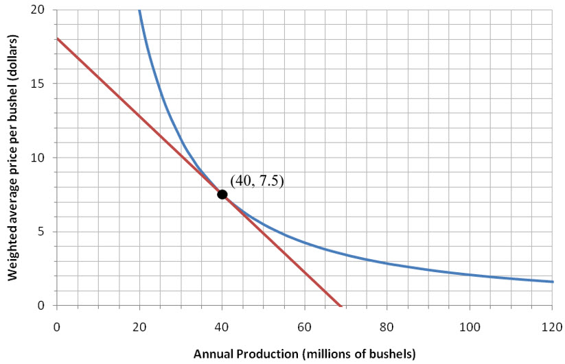
Figure 5 – The demand function for oat production (blue) with the tangent line (red) at a production level of 40 million bushels.

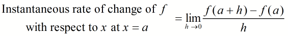
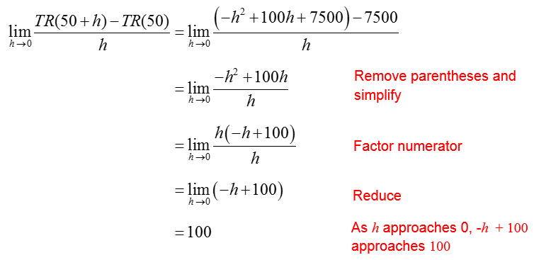
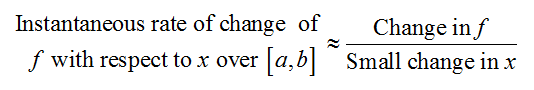
As the change in production level was decreased, the secant line looked more and more like the tangent line. At the same time, the average rate of change of price with respect to a change in annual production became a better and better approximation of the instantaneous rate of change of price with respect to a change in annual production. Recalling that the instantaneous rate of change at a point is also called the derivative at that point, we define the following.

If we zoom in on the point (40, 7.5), we can see that the demand function and the tangent line are almost the same. Since the tangent line looks very much like the function near the point, we often say that the derivative f ′ (a) is the slope of the curve at the point (a, f (a)).

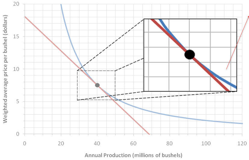
Figure 6 – The demand function for oat production (blue) and the tangent line (red) are almost indistinguishable when we zoom in on the point (40, 7.5).

Example 1    Estimate the Derivative at a Point

The function P = f (Q), pictured below, describes the weighted average price of oats per bushel in dollars as a function of the annual oat production in millions of bushels.

Figure 7 – The weighted price of a bushel of oats as a function of the annual production.

Use a tangent line to estimate the value of the derivative at Q = 40.

Solution The tangent line at Q = 40 is a line that looks most like the function P = f (Q) at that point.

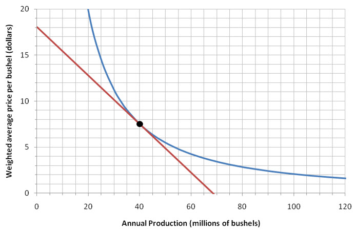
Figure 8 – The demand function for oats (blue) with a tangent line at Q = 40.

The slope of the tangent line at  Q = 40  is equal to  f  ′ (40). If we estimate the location of two points on this line, we can calculate the slope between these points.

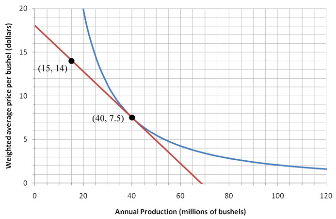
Figure 9 – The tangent line to the demand function with two points estimated.

We locate the points (15, 14) and (40, 7.5) from the graph. The slope m_secant between the points is

Any two points on the tangent line at Q = 40 may be used to estimate the slope of the tangent line. Different points may lead to slightly different estimates for the slope.

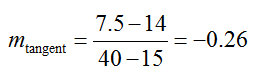
For instance, if we approximate the points (30, 10) and (60, 2.1) on the tangent line, we calculate the slope to be

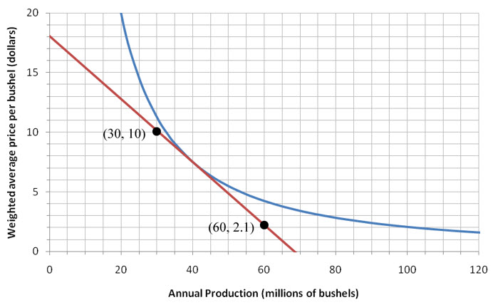
Figure 10 – The tangent line with two different points estimated on the line.

Because we are locating the ordered pairs using the grid on the graph, the values are only guesses at the exact positions. We shouldn’t expect the estimates to be exactly the same. But in this case, careful estimation of the point’s locations leads to similar estimates.

How do you compute the instantaneous rate of change using a limit?

If the quantities being compared in an average rate of change are given by data, we can estimate the instantaneous rate of change using a difference quotient. By using the data nearest the point at which the instantaneous rate of change is desired, we calculate the difference quotient. In the case of the instantaneous rate of change of f with respect to x,

When the quantity in the numerator of the difference quotient is given by a formula, we do not have to settle for an estimate of the instantaneous rate of change. If the quantity in the numerator is given by a function f (x), we can write the average rate of change as

where h describes the magnitude of the change in the denominator. We can use this expression to write a corresponding definition for the instantaneous rate of change. For the instantaneous rate of change, we want the change h to be as small as possible. Although we cannot let this change be zero, we can do the next best thing using a limit.

The instantaneous rate of change of f (x) with respect to x at x = a is

By using a limit as the magnitude of the change h approaches zero, we are able to find the instantaneous rate of change by taking the limit of the average rate of change.

Example 2    Find the Instantaneous Rate of Change

A small toolmaker estimates the annual total revenue TR(x) from selling a quantity of x bearing presses to be

a. Find the instantaneous rate of change of annual total revenue with respect to the quantity of bearing presses sold when 50 bearing presses are sold annually.

Solution Start by rewriting the definition of instantaneous rate of change for the function TR(x) with a = 50,

To calculate the limit, we need to find the revenue function values in the numerator of the difference quotient:

These function values are substituted into the difference quotient to yield

b. Explain what the instantaneous rate of change in part a tells you about how revenue is changing as more bearing presses are sold.

Solution To help us understand what an instantaneous rate of change means in this context, let’s examine the units associated with this rate. For any rate, the units are the units on the dependent variable divided on the units on the independent variable. In this rate, the units on the dependent variable are dollars and the units on the independent variable are bearing presses. So the units on the rate are

An instantaneous rate of

means that selling one additional bearing press will increase revenue by 100 dollars.

Example 3    Find the Instantaneous Rate of Change

Apple is very successful in translating expenditures on research and development into sales of electronic products like Ipods, Iphones and Ipads. Based on data from 2001 through 2010, the annual sales at Apples (in millions of dollars) can be modeled by

where R is the amount, in millions of dollars, spent annually on research and development.

(Modeled from Apple Annual Reports)

a. Find the instantaneous rate of change of sales with respect to research and development spending when annual research and development spending is 1000 million dollars.

Solution For this function, the instantaneous rate of change of sales with respect to research and development spending when 1000 million dollars is spent on research and development is

We can find the function value S(1000) by substituting 1000 into the function,

The function value S(1000 + h) is found by replacing R with 1000 + h,

In simplifying this function value, take care to square the binomial 1000 + h properly. It is very common for students to write incorrectly

Instead, write the square as the product of two binomials and multiply the terms

Using the function values in the definition of instantaneous rate of change leads to

Note that only one term in the limit contains h. As h gets smaller, the term gets smaller and the constant term 40.780 does not change. We compute the limit to be

b. Explain what the instantaneous rate of change in part a tells you about sales and spending on research and development.

Solution The units on the variables help us to determine the units on the instantaneous rate. By dividing the units on the variables,

we get the units on the instantaneous rate of change. An instantaneous rate of 40.780 million dollars of sales per million dollars of research and development means that a one million dollar increase in research and development leads to an increase in sales of 40.780 million dollars. Alternately, we could also say that a one dollar increase in research and development leads to an increase in sales of 40.780 dollars since the factor of millions in the numerator and denominator of the units can be reduced.

How do you estimate the instantaneous rate of change?

The average rate of change of f with respect to x is computed using a difference quotient,

The same difference quotient can be used to compute the instantaneous rate of change of f with respect to x as long as we make the change in the denominator very small. Ideally, we would like there to be no change in x. But this is not possible since it would result in division by zero. However, we can estimate the instantaneous rate of change by making the change in the denominator as small as possible:

The smaller the change in the denominator, the better the estimate is of the instantaneous rate of change.

Example 1    Estimate the Instantaneous Rate of Change

On May 6, 2010, the Dow Jones Industrial Average (DJIA) dropped 998.50 points or 9.2% from the close of trading on May 5, 2010. During the flash crash, the DJIA dropped according to the table below.

At the time, this drop was the largest point drop during any day in history on the NYSE. Twenty minutes after dropping to a level of 9869.62 points, the index recovered around 600 points of the loss. This loss drove the NYSE to develop new trading curbs called “circuit breakers”. These circuit breakers dictate that trading will be halted on any stock on the S&P Index that changes by 10% in a five minute period.

Estimate the instantaneous rate of change of the DJIA 107.0 minutes after 1PM.

Solution The data in the table corresponds to the Dow Jones Industrial Average at various times after 1PM on May 6, 2010. The average rate of change over several different intervals is calculated using the definition of average rate of change,

For instance, the average rate of change of the Dow Jones Industrial Average over the interval [1.7, 107.0] is

An interval of length 105.3 minutes is certainly not an instant or even a reasonable approximation of an instant in time.

The average rate of change of the Dow Jones Industrial Average over the interval [90.0, 107.0] is

Even though the drop in points is not as steep as the previous interval, the average rate of change is greater since the interval is much shorter.

The average rate of change of the Dow Jones Industrial Average over the interval [103.3, 107.0] is

The endpoint on the right of the interval is fixed, but the left endpoint changes in each of these rates. To approximate an instant, we must make the endpoint on the left side of the interval as close as possible to t = 107.0.

The best approximation for the instantaneous rate of change is the average rate of change over the interval [106.7, 107.0],

For this table, an instant is approximated by an interval that is 0.3 minutes long and an instantaneous rate of change of -434.6 points per minute at the time immediately prior to when the Dow Jones Industrial Average began to rise again.

As the average rate of change is computed over smaller and smaller intervals near the lowest point on the graph, it gets more and more negative since the Dow Jones Industrial Average dropped faster and faster before recovering.

How is a limit related to a continuous function?

The definition of continuity is related to limits.

Let’s apply this definition to prove a function is continuous at some point. The state of Arizona uses a piecewise function to calculate the amount of tax T(x) in dollars. For taxable income from $0 to $25,000,

where x is the taxable income. Each piece of this function is a line and each line is continuous. However, do the two lines connect at x = 10000 or is there a discontinuity at that point?

To be continuous, all three conditions of the definition must be satisfied at x = 10000. Condition 1 requires that T(10,000) be defined. According to the function definition,

T(10000) = 0.0259(10000) = 259

This means that an individual with $10,000 in taxable income would pay $259 in tax. So the function is defined at x = 10000.

Condition 2 requires that the two sided limit exist at x = 10000. We will compute the one sided limits and make sure they exist.

The limit from the left and right are both equal to 259 so the two sided limit  exists.

Condition 3 requires that the two sided limit be equal to T(10000). For Condition 2, we showed that

For Condition 1 we found that T(10000) = 259. This means that

The function is continuous at x = 10000.

Figure 3 – The function T(x) is continuous at x = 10000.

As taxable income increases from the lower tax bracket to the higher tax bracket, the amount of tax paid increases continuously. This is due to the fact that the higher rate is only paid on income above 10,000. In effect, an individual in the higher tax bracket pays 2.59% on the first $10,000 in income and 2.88% on income above $10,000 up to $25,000. There is no big jump in the amount of tax paid.

Example 2     Continuous Function

The Basic Plus Plan is a medical insurance plan offered by a self insured trust in Northern Arizona. The total annual cost (in dollars) to an insured person is

where x is the amount of medical charges incurred at the point of treatment.

a.  Prove that BP(x) is continuous at x = 1200.

Solution Check each condition in the definition of continuity at a point.

Condition 1:

BP(1200) = 1200 + 672 = 1872 is defined.

Condition 2:

The one side limits are equal so the two sided limit exists.

Condition 3: Since the one sided limits are both equal to 1872, the two sided limit is also equal to 1872. Additionally, BP(1200) = 1872. So

and the function is continuous at x = 1200.

b.  Prove that BP(x) is continuous at x = 27900.

Solution Check each condition in the definition of continuity at a point.

Condition 1:

BP(27900) = 0.4(27900) + 1392 = 12552 is defined.

Condition 2:

The one side limits are equal so the two sided limit exists.

Condition 3: Since the one sided limits are both equal to 12552, the two sided limit is also equal to 12552. Additionally, BP(27900) = 12552. So

and the function is continuous at x = 27900.

Each of the three pieces in Example 2 is continuous since they are each lines. Since the function is continuous at x = 1200 and x = 27900, the total annual cost increases continuously as the medical charges increase.

Figure 4 – The function BP(x) from Example 2.

What does a continuous function look like?

Let’s compare two different scenarios for the amount of tax paid for taxable incomes between 0 and 25,000 dollars.

In the scenario on the left, the amount of tax increases suddenly as taxable income increases above $10,000. A jump in a function like this is called a discontinuity. It is not possible to graph a function with a discontinuity without lifting your pen off the paper. The graph on the right is a continuous function. It is possible to graph a continuous function without lifting a pen off of the graph.

If taxes in Arizona were to behave like the graph on the left, moving up to higher bracket would cause a jump in tax. However, the graph on the right displays no jump. Both graphs are slightly steeper above 10,000 because of the higher tax rate in that bracket. We’ll see in Question 2 that the amount of tax as a function of taxable income is a continuous function like in the graph on the right.

Functions can be discontinuous for several reasons. As we saw above, a graph can have a jump in it. Other graphs are not defined at some point leading to a discontinuity.

Figure 1 – Each graph is discontinuous at x = a since the functions are not defined at x = a.

In Figure 1, both functions are discontinuous at x = a since the function is not defined there. The graph on the left has a small gap in it. The graph on the right is not defined since there is a vertical asymptote in the graph.

Even if the graph is defined, it may still have a discontinuity.

Figure 2 – Each graph is discontinuous at x = a even though the functions are defined at x = a.

If the point at x = a does not “connect” the pieces of the graph around it, it is not possible to draw the function without lifting a pen from paper. This leads to the discontinuity at x = a.

A function that can be drawn without lifting your pen from the paper is called a continuous function. Graphs of linear and quadratic functions are examples of continuous functions.

Example 1      Discontinuities

For each part, explain why the function is discontinuous at the given point.

a.  f (x) at x = 1

Solution Although the graph has a “kink” at x = 1, that is not the reason it is discontinuous there. The function is discontinuous since the function is not defined at x = 1.

b.  g(x) at x = 3

Solution This function is defined at x = 3, but the pieces of the graph do not connect leading to a vertical gap. This makes the function discontinuous.

c.  h(x) at x = 2

Solution The function is almost connected at x = 2, but the point where they should connect is located in the wrong place. This means we would not be able to graph the function without lifting a pen from the graph. So the function is discontinuous at x = 2.

The idea of drawing a continuous function without lifting pen from paper is not very precise. In the next question, we’ll incorporate limits into a definition of continuity.