How do you evaluate limits at infinity using algebra?
Limits involving rational expressions may be evaluated algebraically. To do this, we need to make an observation.
For any positive real number n,
or
as long as xn is defined.
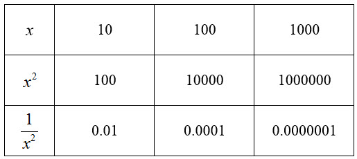
Consider the case where n = 2. A table of values for x2 and 1/x2indicates how the parts of the rational expression behave.
As x grows larger in each limit, the denominator x2 also grows larger. This means the fraction 1/x2 grows smaller and smaller. When evaluating rational expressions, our goal is to simplify the terms in the expression so we can see which terms become smaller and smaller.
We need to be careful about these limits since the second limit is undefined for some values of n. For some values of n like n = 1/2, xn is undefined for negative x values since this amounts to taking an even root of a negative number. In these cases, the second limit as x approaches -∞ is not defined.
Example 4 Evaluate the Limit
Evaluate the limit algebraically:
Solution Start by finding the highest power that appears on x in the denominator. The highest power on the variable in 5x + 4 is one. Divide each term in the fraction by x to this power to yield
For larger and larger values of x, the fractions 1/x and 4/x get smaller and smaller. As these terms approach zero, the constant terms are unchanged. The value of the limit is
The arrows help us to see how the individual pieces drop out as x gets larger.
Example 5 Evaluate the Limit
Evaluate the limit algebraically:
Solution The highest power in the denominator is two. Divide each term in the rational expression by x2 and examine the resulting terms:
Each of the terms in red get small as x increases. This means the denominator approaches 1 but the numerator approaches 0.
Example 6 Evaluate the Limit
Evaluate the limit algebraically:
Solution The highest power of the variable that appears in the denominator is two. Divide each term in the rational expression to give
Each of the terms in red grow smaller and smaller. However, the term in blue grows more and more negative as x grows more and more negative. If the numerator grows more and more negative, the fraction becomes more and more negative. The limit does not exist. Since it does this by becoming more and more negative, we write
How do you evaluate a limit at infinity using a table or graph?
Another type of limit is a limit at infinity. One example is
It is called a limit at infinity because x is written as approaching infinity. Instead of getting closer and closer to a fixed point, the x values get larger and larger. In this case, we find that the farther to the right we move on the graph, the closer the the y values get to the value L. If the limit at infinity is L, the graph of the function f (x) has a horizontal asymptote.
If the y values get very large (negative or positive) as we move to the right on the graph, then the limit does not exist.
Example 1 Find the Limit from a Table
Use a table to evaluate the limit .
Solution To get an idea how the y values behave as x gets large, make a table.
To five decimal places, the y values get closer and closer to 0.40000. Therefore,
Since this limit exists and is equal to 0.40000, the graph of the function has a horizontal asymptote at y = 0.40000.
Example 2 Find the Limit Graphically
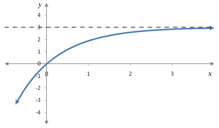
Suppose f (x) is given by the graph below.
Evaluate each of the limits below.
a.
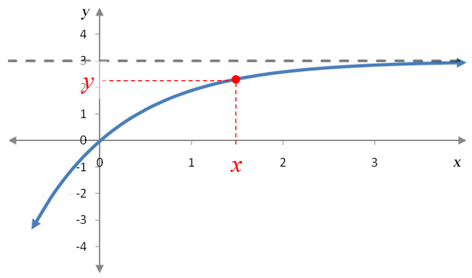
Solution To evaluate this limit, we need to examine y values on the graph as x gets larger and larger.
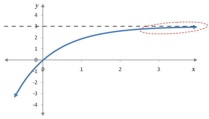
The horizontal asymptote indicates that the graph gets closer and closer to the horizontal line. Let’s locate an x value and its corresponding y value.
Notice that as x values grow larger, the corresponding y value moves vertically closer and closer to 3. In fact, the more the point moves to the right, the closer it gets vertically to y = 3. This tells us that
b.
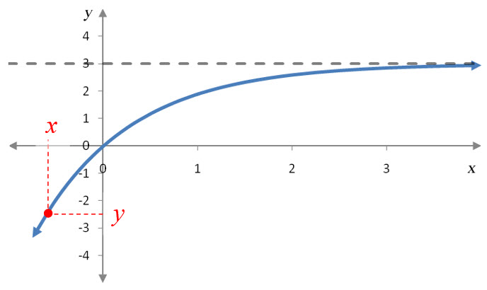
Solution For a limit where x approaches -∞, we let the x values be negative, but larger and larger.
As we move farther and farther to the left on the graph, the corresponding point on the function drops down. This means the y values are dropping and not approaching a fixed value. The limit does not exist. Since the limit does not exist by becoming more and more negative, we write
If the y values were to become more and more positive because the point rises as we move farther to the left or right, we would similarly conclude that the limit did not exist and then use ∞ to indicate how the function values are growing.
For polynomials and other types of functions, we can use the end behavior of the graph to evaluate the limit at infinity.
Example 3 Evaluate the Limit
Evaluate the limit .
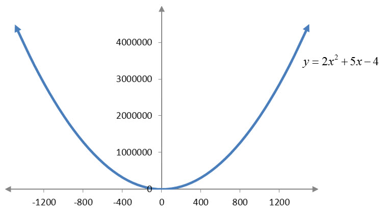
Solution We can use a table or graph to evaluate this limit. Let’s examine both to insure they give a consistent value for the limit.
For x values more and more negative (farther and farther to the left on the graph), the y values grow larger and larger. The y values are not approaching any value so the limit does not exist,
How do you evaluate limits involving difference quotients?
In calculus, we frequently encounter expressions of the form
This type of expression is called a difference quotient. It may appear as part of a limit,
If we try to evaluate this limit by setting h = 0, both the numerator and denominator are zero. This indicates that we’ll need to try to simplify the difference quotient to evaluate the limit.
Example 3 Evaluate the Limit
Evaluate the limit
for f (x) = 5x – 1 and a = 2.
Solution Before attacking the limit, write out the difference quotient with the function and constant a. The two function values in the numerator are
With these values, we simplify the difference quotient:
With this simplification, the limit becomes
Since there is no h in the simplified difference quotient, setting has no effect on the constant. The limit of the constant is the equal to the constant.
As the function becomes more complicated, the algebra required to simplify the difference quotient may be more complicated. Pay careful attention to negative signs and removing parentheses.
Example 4 Evaluate the Limit
Evaluate the limit
for f (x) = x2 – 2x and a = 1.
Solution The function value f (1) is easy to find,
However, the other function value requires several steps to simplify:
Put these values into the difference quotient and simplify to yield,
With the difference quotient simplified, we can evaluate the limit:
We’ll evaluate limits involving difference quotients in Chapter 11. The difficulty in evaluating the limits is not the concept of the limit itself. Instead, the algebra required to simplify the difference quotient is the most challenging aspect. It will require careful attention to algebra details.
For many functions, we can evaluate the limit by substituting the value the variable is approaching into the limit’s expression.
Basic Rule for Evaluating Limits Algebraically
If a function f (x) is made up of additions, subtractions, multiplications, divisions, powers and roots, then the limit as x approaches a may be evaluated by substituting x = a into the function f (x) as long as this function value is defined.
The basic rule applies to one and two sided limits.
Example 1 Evaluate the Limit
Evaluate each of the limits below.
a.
Solution The polynomial is made up of additions, subtractions, powers, and multiplications so we may set x = 2 to find the limit:
b.
Solution The rational expression is made up of additions, subtractions, multiplication and division so substitute t = -1 to find the limit:
c.
Solution As with the earlier parts, substitute the value x is approaching to compute the limit:
d.
Solution When we substitute x = 2 into the rational expression, the denominator is undefined. This means we need an alternate strategy for evaluating this limit.
The basic rule works in many cases. But limits like the one in part d of Example 1 require some extra steps. In this limit, substituting the value x is approaching in the limit results in
The numerator and denominator are both equal to zero. This occurs because the numerator contains a hidden factor of x – 2,
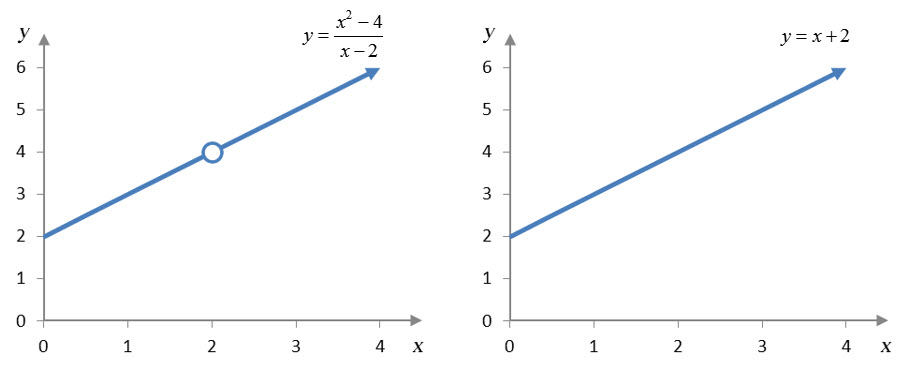
The factors of x – 2 in the numerator and denominator lead to the zeros in the numerator and denominator. Since these factors are the same, we can simplify the rational expression to yield
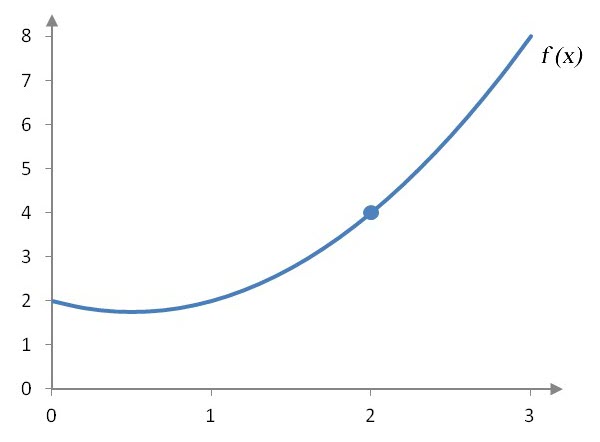
We have written and x + 2 as equal, but in what sense? Let’s examine the graph of each expression.
The graphs are identical except for the point at x = 2. The graph on the left is not defined at x = 2, but the graph on the right is defined there. This has no effect on the limit as x approaches 2. The y values on both functions get closer and closer to 4 as x approaches 2. This means we can simplify the rational expression and then substitute x = 2 into the result. This yields the limit
For limits that give 0/0 when the value is substituted, simplifying the expression often allows the limit to be evaluated by substitution.
Example 2 Evaluate the Limit
Evaluate each of the limits below.
a.
Solution The numerator and denominator are both zero at x = 3. To evaluate the limit, simplify the expression before making the substitution:
b.
Solution When you set x = 0, the numerator and denominator are both zero. To simplify the expression, combine the fractions in the numerator.
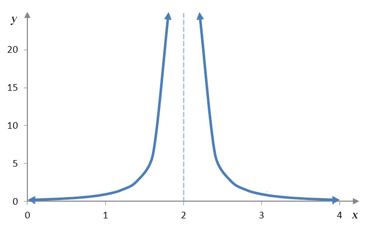
If the expression is undefined, but not because both the numerator and denominator are zero, we fall back to a table or graph to evaluate the limit. For example, in the limit
the denominator is zero when x = 2 is substituted. However, the numerator is not equal to zero. In this situation, a graph allows us to examine the behavior near x = 2.
As xgets closer and closer to 2 from the left or right, the y values grow larger and larger. In terms of the limit, we write
This means the limit does not exist since the y values grow larger and larger.
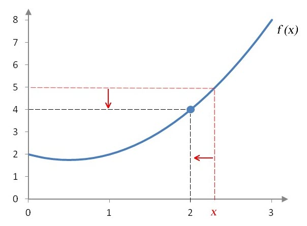
In the question before this one, we used a table to observe the output values from a function as the input values approach some value from the left of right. With a little practice, we can evaluate limits using a graph to find the values of a function. Suppose we have the graph of a function like the one below.
We can use this graph to evaluate the two-sided limit .
As with the limits we calculated from tables, we must evaluate the one-sided limits near x = 2. To calculate the limit
we must examine the graph at x values that are slightly smaller than x = 2.
Figure 1 – As the x values get closer and closer to 2 from values slightly smaller than 2, the y values approach 4.
In Figure 1, a red dashed vertical line is positioned slightly to the left of 2. The height of the line indicates the y value at that xvalue. A red dashed horizontal line locates the y value on the graph. As the vertical line moves closer and closer to 2, the horizontal line gets closer and closer to the y value 4. This means the limit as x approaches 2 from the left is 4 or .
The same strategy allows us to solve the one-sided limit
Figure 2 – As the x values get closer and closer to 2 from values slightly larger than 2, the yvalues approach 4.
The red dashed vertical line in Figure 2 locates an x value slightly larger than 2. The red dashed horizontal line gives the corresponding value on the yaxis. As the vertical line moves closer and closer to 2, the horizontal line moves closer and closer to 4. In other words, for x values closer and closer to 2, the y values are closer and closer to 4. The limit from the right is .
Since the limits from the left and right are both equal to 4, the two-sided limit is also equal to 4,
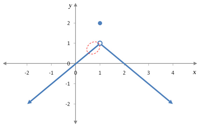
Example 4 Find the Limit Graphically
Suppose f (x) is given by the graph below.
Evaluate each of the limits below.
a.
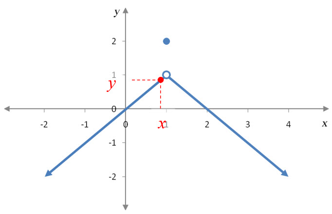
Solution To evaluate this limit, we need to examine y values on the graph as x gets closer and closer to 1 from the left side of 1. This region of the graph is shown in the graph to the below.
Let us locate an xvalue and its corresponding y value in this region.
Notice that as x moves horizontally closer and closer to 1, the corresponding y value moves vertically closer and closer to 1. This tells us that . Notice that the y value at x = 1, f (1) = 2, is not the same as the limit.
b.
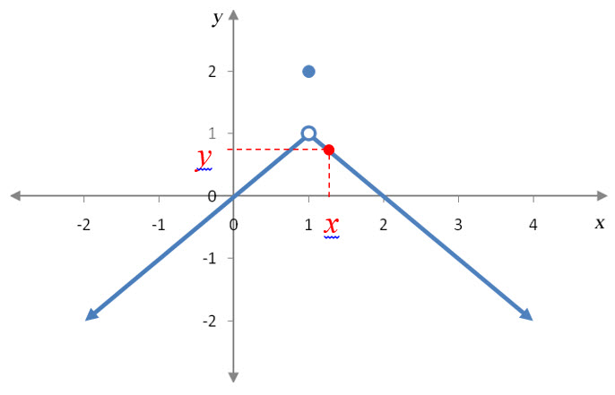
Solution In this one sided limit, the x values are on the right side of 1.
As the point moves to the left towards , the point moves up vertically towards 1. This means that the closer the point gets to x = 1, the closer the y value gets to 1 or .
c.
Solution For the two sided limit to exist, the one sided limits must be equal. In this case they are both equal to 1. Since they are both equal to 1, the two sided limit is also equal to 1,
Notice that none of these limits have anything to do with the fact that f (1) = 2. This is because we are using x values approaching 1, not equal to 1.
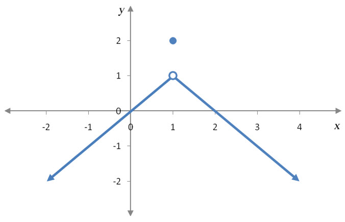
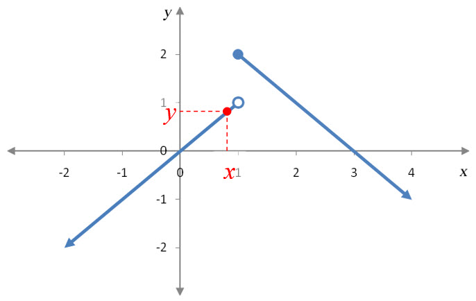
Example 5 Find the Limit Graphically
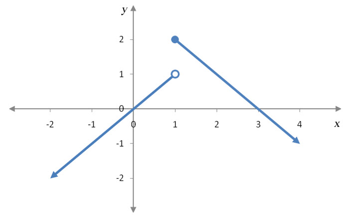
Suppose f (x) is given by the graph below.
Evaluate each of the limits below.
a.
Solution To left of x = 1, the graph looks like the graph in Example 1.
Notice that as x moves horizontally closer and closer to 1, the corresponding y value moves vertically closer and closer to 1. This tells us that .
b.
Solution As the point moves to the left towards x = 1, the point moves up vertically towards 2.
This means that the closer the point gets to , the closer the y value gets to 2 or .
c.
Solution For the two sided limit to exist, the one sided limits must be equal. In this case, they are not equal. From the left side the limit is equal to 1 and from the right side the limit is equal to 2, so
The vertical gap in the graph at is what leads to different values in the one sided limits. In Example 4, there was a horizontal gap at x = 1, but not a vertical gap since the two pieces of the graph come together at x = 1.
In each of these examples, we evaluate the one-sided limits to find the two-sided limit. If the one-sided limits are equal to some value, the two-sided limit is equal to the same value. If the one-sided limits do not match, the two-sided limit does not exist. In the next example, we examine a function for which the one-sided limit does not exist.
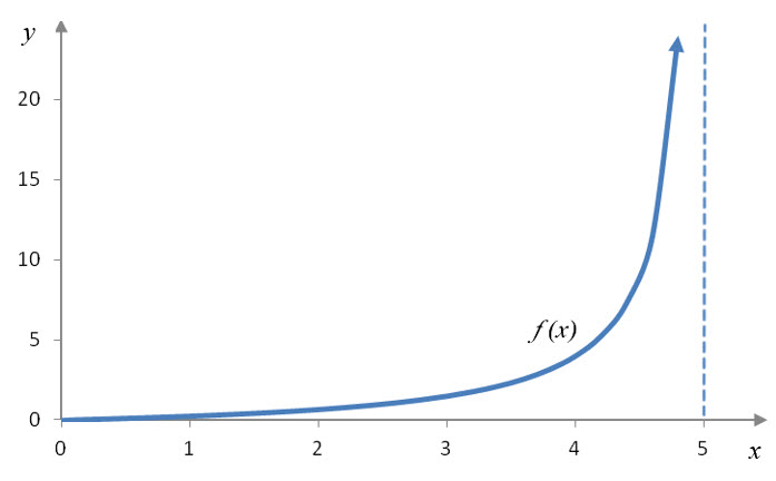
Example 6 Find the Limit Graphically
Suppose f (x) is given by the graph below.
Evaluate the limit .
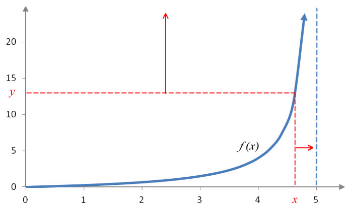
Solution This function has a vertical asymptote at x = 5. The vertical asymptote is shown on the graph as a blue dashed line.
The one-sided limit is a left hand limit. Locate points on the left side of with red dashed lines.
As the vertical line gets closer and closer to 5, the horizontal line gets higher and higher. This indicates that the y values do not get closer to any value as x gets closer to 5 from the left. The one-sided limit does not exist.