Category: Finite Mathematics Ebook

Do all systems of linear equations have unique solutions?

Earlier we examined two systems where the numbers of variables was equal to the number of equations. Often there are fewer equations than variables or more equations than variables. Even in systems where the number of variables initially equals the number of equations, one of the rows may become all zeros, meaning that the equation was unnecessary. In all of these cases, we can still use the strategy from Question 3 to solve the problem.

Example 6    Solve a System with More Variables Than Equations

Solve the system of equations

by transforming its augmented matrix to reduced row echelon form.

Solution This system does not use x, y, and z like earlier examples. However, if we let the first column in the augmented matrix correspond to x₁, the second column to x₂, and the third column to x₃, we can write the augmented matrix for this system as

To put this matrix into reduced row echelon form, we must transform it using row operations to

Since there is no third row, we have no hope of solving for a solution where x₁, x₂, and x₃ are each a unique value. Instead, we’ll be able to solve for x₁ and x₂ in terms of x₃.

The original augmented matrix already has a 1 in the first column and row, so there is no need to put a pivot there. To put a 0 below the pivot, multiply the first row by -2, add it to the second row, and put the result in place of the second row:

The previous row operation not only put a 0 in the first column, but also placed the pivot in the second row and column (very lucky!). To put this matrix into reduced row echelon form, we need to put a zero above the pivot in the second column. Multiply the second row by -1, add it to the first row, and place the result in the first row:

This matrix is in reduced row echelon form, but we can’t read the solution off as we have in earlier examples. If we convert this back to a system of equations, we get

Notice that each of these equations contains x₃ and it is easy to solve for x₁ in the first equation and x₂ in the second equation. If we solve for x₁ and x₂ we get

Although we don’t have specific numbers for each variable, we do have a recipe for finding values. If we choose any value for x₃, we can find the corresponding values for x₁ and x₂. For instance, if we choose x₃ = 100, then

If x₃ = 0, then

Since x₃ can be any number, there are an infinite number of solutions to the system. However, not just any combination of numbers works. Once a value for x₃ is chosen, the equations above must be used to calculate corresponding values for x₁ and x₂. This can be summarized by writing

In this case, we have more variables than equations so we would expect to be able to solve for only some of the variables explicitly. In each row we can solve for a variable explicitly as long as the row is not entirely zeros. Any variables beyond the number of nonzero rows, in this case one, will be values that we can pick. These variables are called parameters. Parameters are variables whose values are arbitrary and can be picked to be anything that is reasonable for the system of equations.

---

 

Example 7    Solve a System with More Equations Than Variables

Solve the system of equations

by transforming its augmented matrix to reduced row echelon form.

Solution The augmented matrix for this system is

To put this matrix into reduced row echelon form, we need to place pivots in the first and second columns and zeros in the rest of these columns.

The entry in the first column and row is a 1 so the pivot is already in place. To put zeros below the pivot,

In the second column and row, we need to transform the 12 to a 1 by multiplying the row by ¹/₁₂:

Now place zeros in the rest of the column,

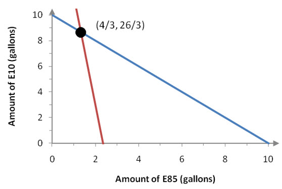
If we convert this matrix back to a system of equations, we find that x₁ = 4 and x₂ = 1. Notice that the last row of the matrix is all zeros and does not contribute to the solution. This means that there are two variables and two nonzero rows so no parameters are needed in the solution.

We can check the solution by substituting (4, 1) into each equation:

Since (x₁, x₂) = (4, 1) satisfies each equation in the system, it is the solution to the original system of equations.

---

 

Example 8    Solve a System with More Equations Than Variables

Solve

by transforming its augmented matrix to reduced row echelon form.

Solution Like the last example, we’ll let the first column in the augmented matrix correspond to and the second column to . The augmented matrix for this system is

To create a pivot in the first row and column, we have two possibilities. We could multiply the first row by ¹/₁₀  or interchange the first and third row. Since interchanging rows does not introduce and fractions into the matrix, we’ll do that to yield

Now we’ll use row operations to fill the rest of the first column with zeros:

To create a pivot in the second row and column, multiply the second row by ¹/₂:

Now use row operations to place zeros above and below the pivot in the second column:

The first two rows in the reduced row echelon form suggest a solution, but the third is problematic. If we write this row as an equation, we get

The left side is simply 0. Since 0 cannot equal 27, this implies that there are no solutions to this system. This system is an inconsistent system.

---

 

These examples illustrate what may happen when there are more equations than variables or when there are more variables than equations. It is possible for the system to have a unique solution as in Example 5. The system may be a system with infinitely many solutions like Example 6 or have no solutions like the inconsistent system in Example 8.

How do you use row operations to determine the reduced row echelon form of a matrix?

To solve a system of linear equations using matrices, we must convert the augmented matrix to another matrix that is in reduced row echelon form.

 

Each of the augmented matrices below is in reduced row echelon form:

When an augmented matrix is in reduced row echelon form, it is easy to find the solution to the system of linear equations.

 

For instance, suppose we have the system of linear equations

This system yields the augmented matrix

Later in this section we see how to get the reduced row echelon form for this matrix,

If we rewrite this matrix as a system of linear equations, we get

Dropping all of the terms with a 0 coefficient leads to the solution, x = 3, y = -2, and z = 1.

We can check to see that these values satisfy the original system to insure it is equivalent to the system of equations corresponding to the reduced row echelon form:

To solve a system of m linear equations in n variables, we will follow a simple strategy.

 

An augmented matrix is transformed to its reduced row echelon form by using three different operations on the rows. These row operations change the entries in the rows without changing the solutions to the corresponding system of linear equations. If these operations seem familiar, it is no mistake. Each operation corresponds to an equation transformation discussed in Section 2.2.

 

Our goal is to use these row operations to transform the original augmented matrix to its reduced row echelon form.

It is helpful to symbolize the row operations to help identify what is being done. If we want to interchange two rows like the first and second, we will write

To symbolize that a row is being multiplied by a constant and replacing another row we use a similar notation. For instance, if we want to indicate that row 1 is being replaced by ¹/₁₀ of row 1 we would write

If we need to indicate that multiples of rows are being added and replacing another row, we would write something like

This particular notation indicates that you are multiplying row 2 by -2 and adding it to row 3. The sum is placed in the third row. Notes like these help us to document our row operations. You are encouraged to adopt the same notes so that you can follow your own work easily.

Example 4    Solve a System of Linear Equations Using Matrices

Solve the system of equations

by transforming its augmented matrix to reduced row echelon form.

Solution The augmented matrix for this system is

The strategy for finding its reduced row echelon form is similar to the strategy for the Elimination Method.

To put this matrix into reduced row echelon form, we’ll work with each column, one at a time. Instead of using equation transformations to change the leading coefficient to a 1, we’ll use row operations to create a 1 in the entry in the first row and first column of the matrix. After placing the 1, we’ll use row operations to put zeros in the rest of the column. This step corresponds to eliminating the first variable in all of the equations except the first equation. We’ll continue through the rest of the columns of the matrix placing ones and zeros in a manner similar to the Elimination Method.

First we’ll use row operations to transform the original augmented matrix to

In each column we’ll use row operations to put the 1 in the column and then continue to use row operations so that the zeros appear below the 1. The 1 is called the pivot in the column.

For this augmented matrix, we could multiply the first row by ¹/₄ or interchange the first and second rows. If we multiply the first row by ¹/₄ and replace the first row with the result we get

The symbols on the left indicate that each entry in the first row is multiplied by ¹/₄.

If we interchange the first and second rows we get

Either row operation puts a 1 at the top of the first column. However, interchanging the rows does not introduce any fractions into the problem, so that is the best row operation to use.

Now that the pivot has been established, we’ll use it to put zeros everywhere else in the column. To put a 0 below the one, multiply the first row by -4 and add the result to the second row. Place the sum in the second row:

The symbols on the left show -4 times the first row of the matrix and the second row below it.  Adding the columns vertically gives the sum that is placed underneath the horizontal bar. The blue arrow indicates where that sum is placed in the matrix.

To put a 0 in the bottom of the first column, multiply the first row in this new matrix by 2 and add it to the third row. Place the sum in the third row:

The first column is in the proper format so now we continue onto the second column. We need to use more row operations to change this new matrix into

Start by putting a 1 in the middle of the second column. This can be done in many ways, but we multiply the second row by –¹/₆ to place the pivot. This gives us

With the pivot in place, we now put zeros in the rest of the second column:

Next we place the pivot in the third column. To put a 1 in the bottom of the third column, multiply the third row by –²/₁₅  and place the result in the third column:

Now that the pivot has been established in the third column, we can place zeros in the rest of the column.

This matrix is in reduced row echelon form and indicates that the solution is x = 3, y = -2, and z = 1.

---

 

Example 5    Solve a System of Linear Equations Using Matrices

Solve the system of equations

by transforming its augmented matrix to reduced row echelon form.

Solution The augmented matrix for this system is

To place a 1 at the top of the first column, interchange the first and second rows. This transforms the original augmented matrix to

A zero is created below the pivot by multiplying the first row by -2, adding this to the second row, and placing the result in the second row. A zero is also created at the bottom of the first column by multiplying the first row by -5, adding this to the third row, and placing the result in the third row. These two row operations yield

In the second column, we need to place a pivot (a 1) in the second row. Multiply the second row by –¹/₅ and place the result in the second row:

Once the pivot is established, we can use it to put zeros in the rest of the column:

With these two row operations, the second column is in the proper format for reduced row echelon form. In the third column, we need to place a pivot in the third row. To do this, multiply the third row by ⁵/₅₄ :

Create zeros above the pivot to put the matrix in reduced row echelon form:

Since the first column corresponds to x, the second column to y and the third column to z, the solution to the original system is x = 1, y = -3, and z = 0.

---

 

In each of the last two examples, the same strategy is used to find the reduced row echelon form. Starting with the first column, we place the pivot in the proper position by interchanging rows or multiplying a row by a constant. Once the pivot is in place, we can multiply the pivot row by a constant and add it to the other rows to put zeros in the rest of the column. By doing this in each column, we can efficiently get the reduced row echelon form and the solution to the system of linear equations.

How do you form an augmented matrix from a system of linear equations?

The entries in a matrix are not just random values without meaning. In general, the rows and columns in a matrix have labels that help you to match numbers with an application. For an augmented matrix, the rows in a matrix correspond to the equations in a system of linear equations. The columns match with the variables and constants in each equation. The augmented matrix that corresponds to the system of linear equations

is

For a system to be written as an augmented matrix, all of the variables in the system must be on one side of the equal sign and in the same order for each equation. The constants must be on the other side of the equal sign.

If we rewrite the system as

we see that the coefficients and constants in the system match with the entries in the augmented matrix. The dashed line between the second and third columns separates the variables from the constants in the system of equations. On the left side of the dashed line are the coefficients of the variables and on the right sides are the constants from each equation,

Following this template, we can write any system of linear equations as an augmented matrix or any augmented matrix as a system of linear equations.

Example 2    Convert a System to an Augmented Matrix

Write each of the systems of linear equations as an augmented matrix.

a.  

Solution Since this system has two equations, the augmented matrix must have two rows. There are two variables and constants in the system so we need three columns in the augmented matrix. We’ll match the first column to the coefficients of x, the second column to the coefficients of y and the third column to the constants. This leaves us with the augmented matrix

b.  

Solution Since there are three equations in the system the augmented matrix needs to have three rows. Although each equation does not have three variables, there are a total of three variables in the system. This means that there must be four columns in the augmented matrix. The last column will correspond to the constants in the system. The augmented matrix is

If a variable is missing from an equation, the augmented matrix contains a 0 in the row and column that matches the equation and missing variable.

c.  

Solution The first equation has the appropriate form to convert into an augmented matrix. The variables are on the left side and the constants are on the right side of the equals sign. However, the second equation has variables on both sides of the equal sign. To convert the second equation to the proper format, remove the parentheses

 

and move all of the variables to the left side,

Replace the second equation with this equivalent equation to give

If we let the first column correspond to x₁, the second column correspond to x₂, and the third column correspond to x₃, the augmented matrix is

---

 

Example 3   Convert an Augmented Matrix to a System of Equations

For the augmented matrix,

write the corresponding system of linear equations with the variables x, y, z.

Solution The three columns to the left of the dashed lines must correspond with the three given variables, x, y, and z. The numbers in each row to the left of the dashed line are the coefficients in the equation. The numbers to the right of the dashed line are the constants in each equation. The first row of the augmented matrix corresponds to the equation x + z = 6. Since there is a 0 in the second column, no y appears in this equation. The second row of the augmented matrix indicates that 0.5x + y – z = 4. The last row gives the equation 2x – 5y +3z = 0.

The complete system of equations is

---

 

Once a system of linear equations is converted to an augmented matrix, we can modify the augmented matrix to determine each variable. Next we’ll look at a strategy for solving the system of equations using the augmented matrix.

What is a matrix?

A matrix is simply a table of numbers enclosed by a set of square brackets. These numbers may correspond to inventory levels, production quotas, or almost anything. We specify the size of a matrix by giving the number of rows and columns in the matrix.

 

The plural of matrix is matrices. The size of a matrix is always listed as row by column. Shown below are several matrices of various sizes.

Any matrix with only one row is also called a row matrix. The matrix in the center is an example of a row matrix. A matrix with only one column is called a column matrix. The matrix on the far right is an example of a column matrix.

Capital letters are used to name matrices. For instance, we might name the 3 x 2 matrix given above with the letter A,

The individual entries in the matrix are denoted by the corresponding lower case letter with a subscript. The number 4 in the third row and first column is called a₃₁ and the number -1 in the second row and second column is called a₂₂. In fact, we can match any entry to its name using the lowercase letter matching its name with a subscript. In general, a_mn is the entry in the m^th row and n^th column.

Example 1    Find the Matrix Entry

For the matrices

find the entries indicated in each part.

a.   b₁₂

Solution Let’s examine the matrix entry in detail.

The entry in the first row and second column of the matrix B is 0.75.

b.   c₂₁

Solution The entry in the second row and first column of C is 3.

c.   b₃₁

Solution This entry matches with the number in the third row and second column of B. Since B only has two rows, does not exist for the given matrix B.

 

How do you set up and solve an application involving a system of equations in two variables?

In section 2.1, we examined how the equilibrium point for the dairy industry could be found from the demand and supply functions from Chapter 1. In that section, we used a graph of the functions to locate the equilibrium point. The Substitution Method and Elimination Method can also be used to find the equilibrium point algebraically.

Example 5    Use the Substitution Method to Find the Equilibrium Point

The demand and supply functions for the dairy industry are described by

Use the Substitution Method to find the equilibrium point for this system of equations.

Solution Since one of the equations (in this case both) is solved for a variable, this system is perfectly suited for the Substitution Method. Substitute ³/₉₅ Q for P in the demand function,

Now solve the equation for Q:

Either equation can be used to determine the corresponding value for P. If we substitute Q = 95 into the supply function, we get

The equilibrium price of $3 per gallon corresponds to a quantity of 95 thousand gallons of milk. At this price, suppliers are willing to supply 95 thousand gallons of milk and consumers are willing to buy 95 thousand gallons of milk.

---

 

We can also locate this equilibrium point using the Elimination Method.

Example 6    Use the Elimination Method to Find the Equilibrium Point

The demand and supply functions for the dairy industry are described by

Use the Elimination Method to find the equilibrium point for this system of equations.

Solution To use the Elimination Method, we must place all of the variables on one side of the equation and the constants on the other side.

This gives the equivalent system

The leading coefficient of the first equation is a 1, so we proceed to eliminating P from the second equation. To do this, multiply the first equation by -1 and add it to the second equation:

The fraction in the sum may look a bit strange, but it comes from converting the decimal to a fraction and adding the fractions:

Replace the second equation with the new second equation to obtain an equivalent system of equations:

Multiply the second equation by the reciprocal of ⁷⁷⁵/₉₅₀₀ to make the leading coefficient a 1,

This helps us to write the system of equations as

To eliminate Q from the first equation, multiply the second equation by ³/₉₅ and add it to the first equation:

Replace the first equation with this sum to yield the solution . This tells us that the equilibrium point is at 95,000 gallons of milk and a price of $3 per gallon.

---

 

The equilibrium point is at the same values when we solve the system of equations by the Substitution Method or the Elimination Method. In general, you’ll solve for the equilibrium point with only one of these methods.

We have looked at several examples of setting up a system of equations from an application and then solving the resulting system. We have broken the process up into several parts and illustrated each part individually to make them easier to understand. In reality, problems are usually not all that tidy. In the following example we’ll solve a problem involving a system of equations in two variables. Our strategy for doing this is fairly straightforward.

 

Example 7    Mixing Ethanol Blends

Flex fuel vehicles are designed to operate on a gasoline-ethanol mixture. This gasoline-ethanol mixture is called E85 and is 85% ethanol and 15% gasoline. Flex fuel vehicles perform almost identically to gasoline powered vehicles. Since E85 is less expensive than gasoline, it would appear that that flex fuel vehicles would be the wave of the future. However, the energy content of E85 is less than that of gasoline so flex fuel vehicles get worse mileage than gasoline powered vehicles. In general, the higher the percentage of ethanol in the fuel, the worse the mileage is.

A recent study determined that several vehicles designed to run on gasoline are able to run well on gasoline-ethanol blends. In tests using E10 (10% ethanol), E20 (20% ethanol) and E30 (30% ethanol), the cost per mile traveled by vehicles using the three blends was lowest for vehicles using E20 or E30. Because of these results, gasoline stations around the country are beginning to sell several blends of ethanol to cash in on this result. A gasoline station in Rapid City, South Dakota carries three blends, E10, E20, and E85. The cost per gallon of each of these fuels is shown in the table below.

A customer wants to purchase 10 gallons of E20. The customer could simply purchase the 10 gallons at $2.68 per gallon. Or the customer could blend their own E20 using the available E10 and E85. How many gallons of E10 and E85 would the customer need to blend in their 10 gallon tank to effectively have E20? Would it be cheaper to blend E10 and E85 or to simply pump E20?

Solution In this problem, we need to compare the cost of pumping 10 gallons of straight E20 to the cost of a specific combination of E10 and E85 that will yield 20% ethanol.

It is straightforward to calculate cost of each type of fuel,

cost = ( cost per gallon ) ( number of gallons )

For instance, 10 gallons of E20 would cost

The key question is to determine if a blend of E10 and E85 would be cheaper. How much of each type of fuel would be needed to fill the tank and result in a mixture that is 20% ethanol? We’ll start with two variables, one to represent the amount E10 in gallons and another to represent the amount of E85 in gallons:

E10: amount of 10% ethanol fuel in gallons

E85: amount of 85% ethanol fuel in gallons

Writing out this description is key to our strategy. Not only does it help you to focus on what the unknowns are, but it also includes the units, gallons.

The problem includes copious amounts of information. However two pieces of information relate to the variables. First of all, the customer needs to fill a 10 gallon tank with a combination of two fuels. Since the variables represent the individual amount of fuels, the sum of the variables corresponds to the total amount of fuel,

The second important piece of information is that the mixture of fuel must contain 20% ethanol. For a 10 gallon tank, the amount of ethanol is 20% of 10 gallons or ( 0.20 )( 10 gallons ) = 2 gallons. This ethanol will come from the E10 which is 10% ethanol and the E85 which is 85% ethanol. By multiplying the percent times the gallons of fuel, we can determine how much ethanol is in the fuel. For instance 8 gallons of E85 and 2 gallons of E10 would have

A mixture of 10 gallons of fuel with 7 gallons of ethanol would be a 70% mixture. This is clearly way too much ethanol. However, we could construct a table with differing amounts of fuel to help us determine the solution:

As the amount of E10 is increased and the amount of E85 is decreased, the total amount of ethanol in the mixture drops. Based on the table, the amount of E10 must be between 8 and 9 gallons and the amount of E85 must be between 1 and 2 gallons. It is unlikely that we could find the exact amounts of each type of fuel by expanding the table.

However, we can replace the amounts of fuel with variables that represent these amounts to give the equation

This gives us two equations in two variables that we can solve by the substitution method or the elimination method.

For this example, we’ll solve the system

Solve the first equation for E10 to yield E10 = 10 – E85. Substitute this expression into the second equation to obtain

Solve the equation for E85:

Now that we know that we’ll need ⁴/₃ gallon of E85, we can use the first equation to find the amount of E10:

Now let’s find the cost of this blend,

Compared to pumping 10 gallons of E20 (for a total of $26.80), pumping a blend of E10 and E85 (from the same pump!) saves about 11 cents.

How does this match the graph of each equation?

Figure 4 – By solving each equation for E10, we can graph E10 = 10 – E85 (blue) and E10 = 20 – 8.5 E85 (red) to see that the point of intersection is at the correct ordered pair.

Before moving on, we need to make sure the solution makes sense. In the table we created earlier, we noted that the amount of E10 had to between 8 and 9 gallons. Since ²⁶/₃ ≈ 8.67, our solution is consistent. The amount of E85  is 4/3 ≈ 1.33 which is between 1 and 2 as expected.

---

Review the steps we outlined for the strategy. Careful examination reveals that the solution above includes all six of the steps for solving an application.