Category: Finite Mathematics Ebook

How do you solve a system of three equations in two variables?

To solve a system of three equations in two variables, we extend the Substitution and Elimination Methods introduced earlier. A third equation in two variables simply adds a third line to the system. A solution to the system is an ordered pair that solves all of the equations in the system.

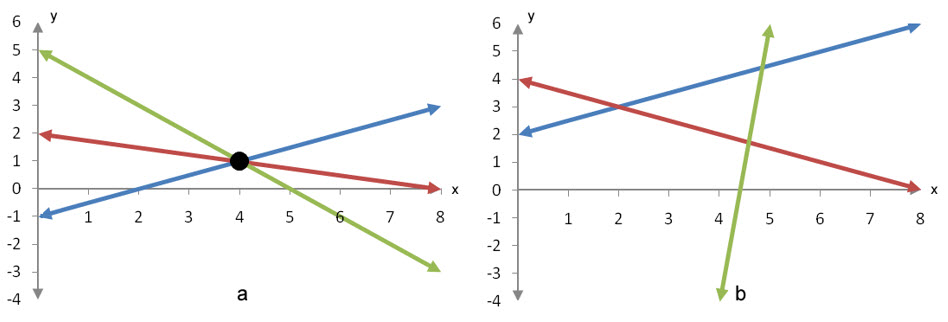
Figure 3 – Two systems of three equations in two variables. In Figure 4a, the solution to the system is (4,1). In Figure 4b, there is no solution since all three lines do not intersect at a single point.

Graphically, this is a point of intersection where all of the lines intersect. In Figure 3a, three lines are graphed corresponding to the three lines in a linear system. All of the lines intersect at the point (4, 1) which means it satisfies each of the equations in the system. If you consider only two of the lines in the system and use the Substitution Method or the Elimination Method, the resulting solution will also satisfy the third line in the system.

The system in Figure 3b has several points, such as (2, 3), where two of the lines in the system intersect. If you use the Substitution Method or the Elimination Method on these two lines, you would find a solution of x = 2 and y = 3. However, if this ordered pair is substituted in the other equation in the system, it will not be satisfied. This means that there is no ordered pair that satisfies all three equations simultaneously so the system is inconsistent.

Example 3    Find the Solution to the System

Solve the system

Solution Although we could use the Substitution Method to solve this system, the Elimination Method will be used in this example since it generalizes to larger systems much more easily. The leading coefficient of the first equation is already a 1, so we need to eliminate x from the other two equations.

Replace the second and third equations in the original system of equations with these new equations to give

Multiply the second equation by ¹/₁₂ to give the equivalent system of equations,

To complete the Elimination Method, we need to eliminate y from the first and third equations:

This helps us to write the equivalent system of equations,

The last equation is an identity which means it is always true. The first two equations indicate that the solution to two of the equations is (x, y) = (4,1). This and the identity indicate that this ordered pair also solves the third equation. We can check this by substituting into each equation:

Since (x, y) = (4,1) satisfies each equation in the system, it is the solution to the system of equations. Furthermore, since the first two equation specify a unique solution and not a relationship between the variables, this is the only solution to the original system of equations.

---

 

Example 4    Find the Solution to the System

Solve the system

Solution Start by solving any two of the equations for a solution. The Elimination Method provides a systematic approach for solving this system. To make the leading coefficient on the first equation a 1, interchange the first and third equation to yield

Now eliminate x from the second and third equations:

Replace the second and third equations with these new equations to give an equivalent system of equations,

Multiply the second equation by ¹/₂ to change the leading coefficient of the second equation to a 1. This leaves us with the equivalent system of equations,

Finally, eliminate x in the first and third equations:

Use these new equations to write the equivalent system of equations,

This indicates that (x,y) = (2,3) satisfies two of the equations, but not the third. The third equation is a contradiction. So the system is inconsistent and has no solutions. If we substitute into the original system of equations, we can discover which equations are satisfied and which are not:

---

 

The strategies in Example 3 and 4 can be applied to a system of any number of equations in two variables. If you use the Substitution Method, find the solution to two of the equations and then check it in each of the other equations. A solution to the system will satisfy all of the equations in the system. If the solution from any two equations does not work in all of the other equations in the system, the system does not have any solutions. If you use the Elimination Method, follow the strategy and look for the transformations to yield new equations that are contradictions (the original system has no solutions) or identities (the original system has many solutions). Remember, contradictions are equations like 0 = 27 that are never true and identities are equations like that are always true.

Does every system have a unique solution?

For systems of two equations in two variables, it is possible to draw two lines that do not intersect. A system like this is called an inconsistent system.

Figure 2 – The graphs of parallel lines do not cross.

For an inconsistent system, there are no ordered pairs that simultaneously solve both systems since the graphs never cross. On a graph this may be difficult to diagnose. Two lines that are almost parallel might be indistinguishable from two lines that are parallel. Luckily when we attempt to find a solution with the substitution method or the elimination method, parallel lines are easy to distinguish from lines that are almost parallel.

Example 1    Determine if a System of Equations is Inconsistent

Decide if the system of equations

is inconsistent by attempting to solve the system.

Solution This is the same system we solved in Section 2.1 Example 4. In that example, we graphed each equation and showed that lines were parallel. In this example, we’ll solve the equations by one of two possible strategies, substitution or elimination. We’ll look at each of these strategies to ensure that you understand how you could solve either way.

Substitution Method

It is easy to solve for x in the first equation by adding 3y to both sides of the equation. This yields

x = 3y + 27

Now replace the x in the second equation with 3y + 27:

-0.25 (3y + 27) + 0.75y = 6.75

We can simplify the left hand side of the equation to give us

Notice that the variable has dropped out of the equation. The resulting equation makes no sense since -6.75 cannot equal 6.75. This contradiction tells us that this system has no solutions.

Elimination Method

The leading coefficient in the first equation is a 1, we begin by eliminating x in the second equation. Either variable can be chosen, but in this system it is easier to eliminate x. Multiply the first equation by 0.25 and add it to the second equation:

Notice that y is eliminated at the same time x is eliminated. The sum of these equations results in a contradiction so the system has no solutions.

In each method, solving the system results in a contradiction. Contradictions such as these indicate that there are no solutions.

---

So far we have seen that a system may have a unique solution (one ordered pair solves the system) or no solutions at all. Other systems of equations have nonunique solutions. For these systems, there are many ordered pairs that satisfy each equation in the system. We may still use the Substitution Method or the Elimination Method to solve systems of equations with nonunique solutions.

Example 2    Does the System of Equations have a Unique Solution?

Decide if the system of equations

has a unique solution by attempting to solve the system.

Solution As in the previous example, we can solve this system algebraically using the Substitution Method or the Elimination Method. In this example we’ll solve the system with both methods. In general, you only need to use one of these strategies to solve the system.

Substitution Method

This system is ideal for the Substitution Method since the first equation is already solved for one of the variables. Substitute -2x + 10  in place of y in the second equation to yield

Now simplify the left hand side to solve for x:

All the variables have dropped out and the resulting equation is always true. This signals that there is not a unique solution to the system. Many ordered pairs will satisfy both equations in the system of equations.

Elimination Method

To use the Elimination Method, we need to have all of the terms with variables on one side of the equals sign and the constant terms on the other side. The first equation does not have this format so add 2x to both sides of the equation to give

2x + y = 10

Replacing the first equation in the system with this equivalent equation leads to

We could multiply the first equation by ¹/₂ to make the leading coefficient a 1. But the second equation has a leading coefficient of 1 so we’ll interchange the equations to give an equivalent system,

To eliminate x from the second equation, multiply the first equation by -2 and add it to the second equation:

This new equation helps us to rewrite the system as the equivalent system

As in the Substitution Method, when all of the variables drop out and leave us with a true statement, there is not a unique solution. Since there is not an equation that specifies y to be a unique number, it can be chosen to be any number. Then the corresponding x value is found using the other equation in the system, . The easiest way to do this is to solve for x first to give .

We could also use the other equation in the original system, y = -2x+10, to find solutions to this system. In this case, we could specify x to be any number. Then the corresponding value of y is found from the equation y = -2x + 10.

In either case, the ordered pairs we find lie on a line. Any ordered pair on that line is a solution to the system. To locate points on this line, simply substitute a value for x in the equation y = -2x + 10 or substitute a value for y in the equation . We can pick any reasonable value for x and use the equation y = -2x + 10 to find the corresponding value for y:

We can also pick a value for y and use the equation  to find the corresponding value for x:

In either case, we find the exact same ordered pairs are solutions to the system. To write this solution formally, we say that the solution is all ordered pairs (x, y) where y = -2x + 10 and x is any real number. You can think of each ordered pair corresponding to an arbitrary x value and a y value that is calculated from the equation of the line. Or you can think of each ordered pair corresponding to an arbitrary y value and an x value that is calculated from the equation of the line.

How do you solve a system of linear equations?

There are two basic strategies for solving a system of two linear equations and two variables. In each strategy, one of the variables is eliminated allowing us to solve for the remaining variable. These two strategies are called the Substitution Method and the Elimination Method.

Although the Substitution Method may be used to solve a system in any number of variables with any number of equations, we’ll use the Substitution Method for systems of two equations in two unknowns. The Elimination Method may also be used to solve systems of equations in two variables. Additionally, the Elimination Method can easily be scaled up to solve systems of equations with more than two variables.

Example 1    Find the Solution to the System

Solve the system of linear equations

using the Substitution Method.

Solution Using the first equation, solve for x. Add 2y to both sides to yield x = 2y – 5. Replace x with 2y – 5 in the second equation and solve for y:

The value for x is found by substituting y = 2 into the equation x = 2y – 5. This gives x = -1. The solution to the system is (x, y) = (-1, 2).

We can check the solution by substituting the solution into the original system:

Since the ordered pair makes both equations true, we have found the solution to the system.

---

In Example 6 of section 2.1, we found the point of intersection of the system of equations

Recall that the first equation describes the total cost Y for operating a dairy with Q cows. The second equation describes the total revenue Y for a dairy with Q cows. When the total revenue and total costs are equal, the business is at the break-even point. This point can be found graphically by locating the point of intersection on the total cost and total revenue graphs. The same point can be found algebraically using the Substitution Method. This strategy is ideal for this system since one (in this case, two) of the equations in the system is in slope-intercept form and solved for a variable.

Example 2    Dairy Break-Even Point

Solve the system of equations

using the Substitution Method.

Solution Since each equation is solved for a variable, Y, we can replace that variable in the first equation with the equivalent expression from the second equation:

3547Q = 2890.8Q + 68688

To solve for Q:

The corresponding value for Y is Y ≈ 3547(104.68) ≈ 371,299.96. This tells us that break-even quantity is 104.68 cows and yields revenue and costs of about $371,299.96.

---

When it is not easy to solve for a variable, the Elimination Method can be used to eliminate a variable from the system of two equations. The Elimination Method relies upon the concept of equivalent systems of equations. Two systems of equations are equivalent if they share the same solution. A system of equations can be transformed to an equivalent system of equations using equation transformations.

Using these three transformations, we can change a given system to a simpler system whose solution is easy to identify. These transformations can be applied to a system of equations in two variables or more than two variables.

Example 3    Find the Solution to the System

Solve the system of linear equations

using the Elimination Method.

Solution This system already has the variables on the left side of the equations and the constants on the right side of the equation. The terms are aligned so that each variable on the left side appears below terms with the same variable.

To make the coefficient of x in the first equation a 1, multiply the first equation by the reciprocal of 5 or ¹/₅

If we replace the first equation with this multiple of the first equation, we get the equivalent system of equations

Now that the leading coefficient in the first equation is a 1, eliminate x from the second equation. To do this, replace the second equation with -2 times the first equation added to the second equation:

Replace the second equation with this sum to yield the equivalent system of equations,

The leading coefficient of the second equation is – ²⁴/₅. To change the leading coefficient to a 1, multiply the second equation by – ⁵/₂₄ :

Put this equation in place of the second equation to give the equivalent system of equations,

To complete the problem, we need to eliminate y in the first equation. Multiply the second equation by – ²/₅ and add it to the first equation:

Replace the first equation with this sum to yield an equivalent system of equations,

Since this system is equivalent to the original system of equations, the solution to the original system of equations is (x, y) = (⁶/₅, – ⁵/₂) .

---

Example 4    Find the Solution to the System

Solve the system of linear equations

using the Elimination Method.

Solution This system of three equations has three variables and each equation does not have all three variables. However, this does not change the strategy introduced earlier. Before we can transform the equations to eliminate variables, we need to move all variable terms to the left side of the equations and constants to the right side of the equations. Subtract from both sides of the third equation and align the variables to give the system

Notice how each variable lines up vertically. If a variable is missing, we simply insert a space to insure all variables are properly positioned.

The leading coefficient in the first equation is a 1, so we need to eliminate x from all other equations.

To eliminate x from the third equation, multiply the first equation by 3 and add it to the third equation:

Replace the third equation in the system of equations with this sum,

Multiply the second equation by the reciprocal of its leading coefficient, ¹/₂:

Put this equation in place of the second equation to give an equivalent system of equations,

To eliminate y from the first and third equations,

Replacing these new equations in the system of equations give the equivalent system,

The leading coefficient of the third equation is changed to a 1 by multiplying the third equation by ¹/₅,

Replace the third equation with this new equation to give

To finish the transformations, we must eliminate z from the first and second equations:

Replacing these new equations in the system leaves us with

Since this system is equivalent to the original system, the solution is (x, y, z) = (-1, 0, 2).

---

The supply and demand curve for the dairy can be written as the system of equations

In this system of equations, the first equation corresponds to the demand function. This line relates the price P to the quantity of milk Q demanded by consumers at that price. The second equation, the supply function, relates the quantity of milk Q that suppliers are willing to supply at a price P. This system is equivalent to the system

that we found for dairies in Chapter 1.

Example 5     Find the Dairy Equilibrium Point

Find the equilibrium point by solving the system of equations

using the Elimination Method.

Solution To solve the system, we need to use equation transformations to change the leading coefficient of the first equation. By multiplying the first equation by ¹/₁₀₀, the leading coefficient becomes a 1:

Replace the first equation in the system with the new equation to yield an equivalent system of equations:

Now we must eliminate P from the second equation. The sum of -95 times the first equation added to the second equation is

Replace the second equation in the system with this new equation:

The leading coefficient of the second equation is changed to a 1 by multiplying both sides of the equation by – ⁴/₃₁:

Replace the second equation with this new equation to give an equivalent system,

Finally, eliminate Q from the first equation.

Placing this equation in the system, we get

So the solution to this system is (Q, P) = (95,3) meaning that at a price of $3 per gallon the quantity demanded by consumers is 95 thousand gallons.

Where do systems of equations come from?

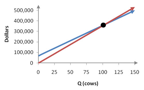
In Examples 4 and 5 of section 1.2, we found the total cost C(Q) and the total revenue R(Q) for a dairy as a function of the number of cows, Q. The total cost function, C(Q) = 2890.8Q + 68688, and the revenue function, R(Q) = 3547Q, are graphed in Figure 5.

Figure 5 – Revenue and cost functions for the dairy.

As the number of cows at the dairy is increased, the cost to maintain the dairy and the revenue from dairy products both increase. In the window shown in Figure 5, the two graphs do not intersect. But the revenue function has a slope of 3547 and the cost function has a slope of 2890.8. Since the revenue function is steeper than the cost function they will eventually intersect.

We can form a system of equations whose solution corresponds to the point of intersection by replacing the function notation with a variable. Let Y represent the amount of money in dollars and use Y to replace both R(Q) and C(Q). This is reasonable since both functions output amounts of money in dollars. The system

allows us to see the relationship between the revenue and cost for a business. By graphing this system, we can interpret what the point of intersection means in the context of the dairy and other types of businesses.

Example 6    Find the Point of Intersection for the Dairy

Graph the system of equations

to find the solution to the system.

Solution Each equation in the system is solved for the dependent variable Y and can be graphed directly.

Figure 6 – The system of equations representing the cost (blue) and revenue (red) of a dairy.

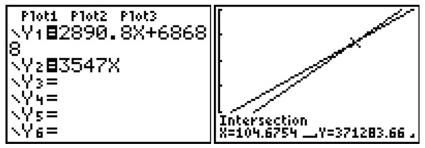
To find an estimate of the location of the point of intersection, we can use a graphing calculator or other type of technology.

Figure 7- Screenshot on a graphing calculator of the system of equations in Example 6.

The point of intersection is at Q ≈ 104.6754 and Y ≈ 371283.66. This tells us that at approximately 104.6754 dairy cows, the total cost of maintaining the herd is about $371,283.66 and the revenue generated by the herd is about $371,283.66. At this point, the total cost and revenue are exactly the same.

A break-even quantity of approximately 104.6754 dairy cows leads to an interesting point. Is it possible to have 0.6754 of a dairy cow? The quantity of cows Q must take on non-negative integer values. The dairy owner will have either 104 cows or 105 cows. Let’s examine the costs and revenue at each of these herd sizes.

At a herd size of 104,

the costs are slightly higher than the revenue by about 369,331,20 – 368,888 or 443.2 dollars. This indicates that the dairy would be losing money. In terms of profit, the dairy has a negative profit since the costs are greater than the revenue.

At a herd size of 105,

the revenue is slightly higher than the cost by about 372,435 – 372,222 or 213 dollars. The dairy is making money since the profit is $213 at this herd size.

Neither herd size results in the revenue equal to the cost. For realistic herd sizes, the revenue and costs are not exactly equal. However, a herd size of 105 is closer to the point of intersection.

---

 

The point at which a business’s costs and revenue are equal is called the break-even point. As demonstrated in Example 6, this point can be found by solving a system of equations consisting of a revenue equation and a cost equation.

In specifying a break-even point, we may find that the point of intersection is at an unrealistic value due to the nature of the items being produced. A complete analysis should examine the break-even point as well as realistic values for the variable near the break-even point.

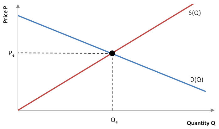
We can also examine where other graphs intersect to find business-related quantities. In Chapter 1, we introduced supply and demand functions. The supply function S(Q) represents the price at which suppliers would be willing to supply Q products. The demand function D(Q) represents the price at which consumers would be willing to buy Q products. In a market, the demand by consumers and the supply by manufacturers may or may not be in balance.

The quantity demanded by consumers may be in perfect balance with the quantity supplied by suppliers. At this price and quantity, called the equilibrium point, consumers demand the exact quantity that manufacturers are willing to supply. On a graph of the supply and demand functions, the equilibrium point is the point of intersection of the two graphs. This ordered pair is labeled (Q_e, P_e), where the subscript refers to equilibrium.

Figure 8 – At the equilibrium point (Q_e, P_e) the quantity demanded by consumers is matched by the quantity that manufacturers are willing to supply.

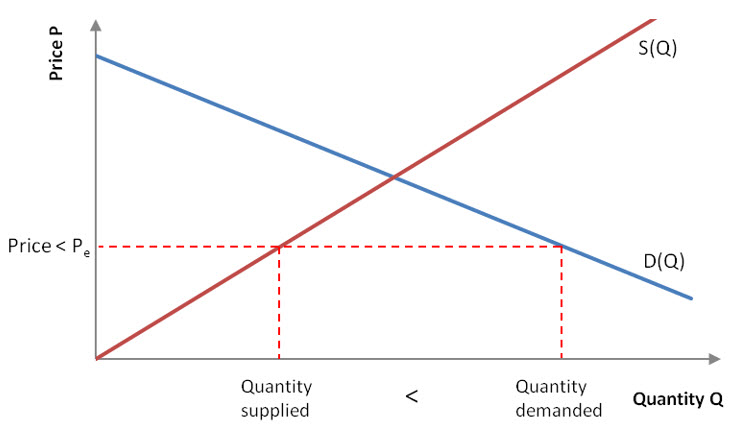
At prices lower than the equilibrium price, the quantity demanded by consumers is larger than the quantity supplied by manufacturers. In Figure 9, the red dashed horizontal line corresponds to a price that is lower than the equilibrium price. When the quantity demanded by consumers is larger than the amount supplied by manufacturers, there is a shortage of the product.

Figure 9 – If the price is below the equilibrium price, the quantity demanded by consumers is greater than the quantity that manufacturers are willing to supply. This results in a shortage of the item on the market.

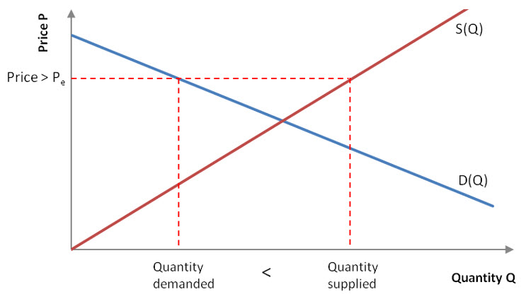
When the quantity that manufacturers are willing to supply is greater than the quantity the consumer is willing to buy, there is a surplus of the item on the market. A surplus occurs when the price of the product is greater than the equilibrium price.

Figure 10 – If the price is above the equilibrium price, the quantity supplied by firms is greater than the quantity that suppliers are willing to supply. This results in a surplus of the item on the market.

A surplus of an item will lead to lower prices since it costs businesses money to keep inventory on hand. The price will tend to lower until the price reaches the equilibrium price. At this point the quantity demanded by consumers and the quantity that manufacturers are willing to supply will be equal.

Example 7      Find the Milk Equilibrium Point

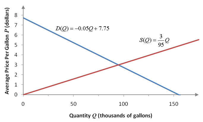
In earlier examples, we found the supply and demand functions pictured below for a small dairy.

Figure 11 – The demand function D(Q) and the supply function S(Q) for the dairy.

Find the equilibrium point for the dairy.

Solution The graph in Figure 11 shows an equilibrium point at roughly (100, 3). To find a better estimate of the equilibrium point, we need to utilize some sort of technology like a graphing calculator. Start by rewriting the functions D(Q) and S(Q) with a variable. Since the output from each of these functions is a price, we’ll use P. The system of equations is

The first equation relates the quantity of milk demanded by consumers to the price. As you would expect, higher quantities are demanded when the price is lower. The second equation relates the quantity of milk that dairy farms are willing to supply to the price. Higher quantities are supplied when the price is high.

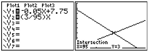
Figure 12 – A screen shot of the system of equations in Example 7. The equilibrium point is at (95, 3).

According to the estimate in Figure 7, at an average price per gallon of three dollars, 95,000 gallons of milk will be demanded by consumers and dairies will be willing to supply 95,000 gallons of milk. Since the demand and supply are in balance, this is the equilibrium point.

What is a system of linear equations?

In many applications there is more than one equation that governs the solution to the problem. For instance, suppose we want to process 100,000 gallons of raw milk into whole, 2%, and 1% milk. Each type of milk sells for $3.49, $4.19 and $4.59 per gallon respectively. The dairy needs $424,000 in revenue from the sale of the milk. If Q₁, Q₂, and Q₃ are the amounts of whole, 1% and 2% milk processed in gallons, the solution to this problem must satisfy

By using the term “satisfy”, we mean that when values are substituted into the variables Q₁, Q₂, and Q₃, the left hand side of each of the equations is equal to the right hand side of the same equation. When the two sides of the equation yield the same values, we say that the values result in a true statement. If the values substituted into the equation result in different values on each side of the equation, we say that the values result in a false statement. There are two equations for this problem since the dairy wants to use all of the raw milk and have $424,000 in revenue from the sales of the processed milk. Any combination that allows the dairy to meet both of these requirements is a reasonable solution to this application.

To check whether there exists a combination of milk products that works, we need to substitute values for the variables into each equation.

Example 1     Do Specific Combinations Solve Both Equations?

For each part below, determine if the combination of milk is a solution to the equations

where Q₁, Q₂, and Q₃, are the amounts of whole, 1% and 2% milk processed in gallons.

a.  50,000 gallons of whole milk, 50,000 gallons of 1% milk and no 2% milk.

Solution For this combination of milk, we have Q₁ equal to 50,000, Q₂ equal to 50,000, and Q₃ equal to 0. If we substitute these values into the first equation, we get

50,000 + 50,000 + 0 = 100,000   TRUE

Since the left hand side of the equation is equal to 100,000, this combination of milk results in a true statement and combines to give the proper amount of milk. However, when we put this combination of milk products in the second equation, we get

3.49(50000) + 4.19(50,000) + 4.59(0)  424,000  FALSE

The left hand side of the equation simplifies to 384,000 to yield a false statement. This combination of milk products does not solve the second equation. This combination solves the first equation so the amounts total to 100,000 gallons of milk, but does not solve the second equation. The amount of revenue from the sales does not equal $424,000.

b.  10,000 gallons of whole milk, 60,000 gallons of 1% milk and 30,000 gallons of 2% milk.
Solution Put the values Q₁ = 10,000, Q₂ = 60,000, and Q₃ = 30,000 into each equation:

yields two true statements. Since this combination makes each equation true, we know that it gives both the proper amount of milk and the proper revenue.

---

For this set of equations, each variable was raised to the first power so the equations are linear in each variable. When the combination of values solves each of the linear equations, the values for the variables are a solution to the system of linear equations formed by the two equations.

Let’s generalize these ideas to help us understand exactly what a system of linear equations is. A system of linear equations consists of several equations containing variables and constants. Recall that variables are letters or symbols that represent unknown quantities. In any of the linear equations, the variables can vary. Constants are values that do not change in an equation. Constants may be numbers like 3 or –5. Or a constant may be a letter that represents a fixed but unknown number.

As illustrated in Example 1, the equations in a system of linear equations can have any number of variables. It is best to name them in a systematic way. Since we were referring to quantities of milk, the letter Q was useful. There were three variables so subscripts distinguish each type of milk and yield Q₁, Q₂, and Q₃.

For business problems we need to allow for any number of variables representing a variety of quantities. We could use variables without subscripts like x and y, but we would run out of names quickly for most realistic applications. If we use the letter x, n variables are represented by x₁, x₂, …, x_n. Letters representing constants can be handled in a similar manner. We can represent n constants using the letter a as a₁, a₂, …, a_n. The single constant on the right side of a linear equation is represented by the letter k. With these constants and variables, a definition for a linear equation can be written. Keep in mind that there is nothing special about the letters used and any letter could be used in place of a, k or x. However, since a₁, a₂, …, a_n and k are constants, these letters represent fixed values. This makes them different from the variables x₁, x₂, …, x_n which represent values that can vary in the equation.

Two special cases must be noted. Many simple problems involve only two variables. We could write the linear equation as a₁x₁ + a₂x₂ = k, but often the letters a, b, x, and y are used. An equivalent linear equation in two variables is ax + by = k . Similarly, for three variables you can write a₁x₁ + a₂x₂ + a₃x₃ = k or ax + by + cz = k. For more than three variables we run out of letters at the end of the alphabet and resort to subscripts. The key concept is that each term in the equation has first degree. Another way to say this is that the variable in each term is raised to the first power. As long as each term is a first degree term, the equation is called a linear equation.

If we collect several linear equations in the same variables together, we get a system of linear equations.

 

Example 2     Do Certain Values Solve the System of Linear Equations?

The equations

form a system of linear equations since the collection of equations can be written as

Do the values x = 7 and y = 2 solve the system?

Solution To see if the values solve the system, we need to put the values into each equation and make sure both equations are true.

Since both equations are true, the values x = 7 and y = 2 solve the system of linear equations.

---

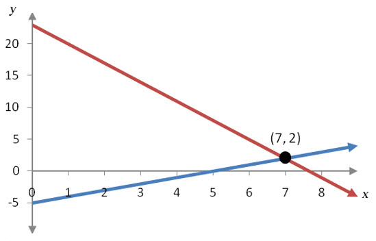
It is convenient to think of this solution in Example 2 as an ordered pair (x, y) and to write the solution as (7, 2). There is a good reason for doing this. The equations in Example 2,

both have graphs that are lines. These lines intersect at the solution to the system of linear equations. The first equation corresponds to a line with a slope of 1 and a vertical intercept of -5. The second line has a slope of -3 and a vertical intercept of 23.

Figure 1 – The two lines corresponding to the system of linear equations intersect at the solution (7, 2).

Graphing each equation is a simple way of estimating the solution to a system of equations. If the system of equations contains only two variables, the solution to the system is the point of intersection of all lines in the system if such a point exists.

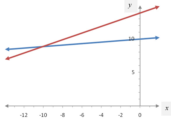
Example 3     Find the Point of Intersection

Find the solution to the system of equations

by finding where the graphs of the equations intersect.

Solution To graph each equation, solve it for y. For the first equation,

To solve the second equation in the system for y,

The system can now be written as

Each of these equations is in the slope-intercept form for a line, y = mx + b. In this form, m is the slope of the line and b is the vertical intercept of the line.

Figure 2 – A graph of the system in Example 3.

It is a good idea to make sure the lines are graphed properly. The blue line has a vertical intercept of 10 and a slope that is small and positive, ²²/₂₀₂ ≈ 0.11. The red line has a vertical intercept of 13.9 and a slope that is larger, ⁵⁰/₁₀₁ ≈ 0.50. Because the slope of the red line is larger than the slope of the blue line, the red line is steeper than the blue line.
Based on the graph in Figure 2, the point of intersection appears to be about (-10, 9). However this can’t be correct since and do not satisfy the two equations in the system.

The best we can say, based on the graph, is that the solution is close to (-10, 9). We’ll need to use a graphing calculator or algebraic techniques to be more precise. However, keep in mind that a graphing calculator will give a better answer, but is still an approximation. Algebraic techniques give the exact answer as long as numbers are not rounded in the process of finding the point of intersection.

---

By substituting these values into the system of equations, we can determine that these values are the exact solution:

When utilizing technology to find a solution, keep in mind that the solution is only an estimate unless the solution satisfies each equation in the system.

Each of the linear systems of equations we have considered has a single point of intersection. You can easily imagine a situation where two lines do not intersect. A system of equations for which the graphs do not intersect has no solutions.

Example 4      Find the Solution to the System of Equations

Solve the system of equations

by graphing both equations on the same graph.

Solution To graph each equation, we need to solve each equation for y.

When each equation is solved for y, we get an equivalent system of equations,

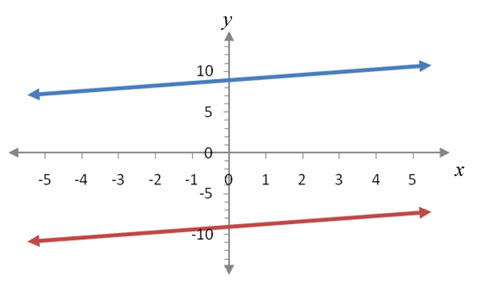
 Figure 3 – A system of equations whose graphs are parallel.

Examining this system, we see that the slope of each line is ¹/₃ and the y intercepts are different. The lines in the system, graphed in Figure 3, are parallel and so the system has no solution.

---

 

Example 5      Find the Solution to the System of Equations

Graph the system of linear equations

to find the solution of the system.

Solution The first equation is already solved for y, but the second is not. Start by solving the second equation for y:

This equation is identical to the first equation so its graph is the same as the first equation. In other words, the two equations are different descriptions of the same line.

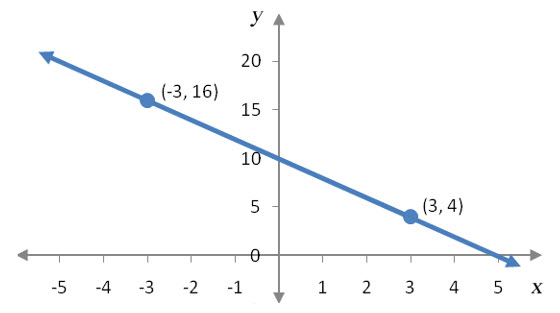
Figure 4 – The graphs of the two equations in Example 5 coincide everywhere along the line.

Any point on the line is a solution to the system of equations. For instance, the ordered pair (-3, 16) is a solution,

as well as the ordered pair (3,4):

We can symbolize this fact by writing the solution as any ordered pair (x, y) such that y = -2x + 10. Since both equations represent the same line, we could also say that the solution is any ordered pair (x, y) such that x + ¹/₂ y = 5.