In section 1.1, we defined a linear function in the variables x and y,
y = mx + b
When the function is written this way, we say “y is a linear function of x”. This means the variable x is the independent variable and the variable y is the dependent variable. The other letters in this equation, m and b, correspond to numbers. For instance, in the equation y = 2x + 3 the value of the constant m is 2 and the value of b is 3. We distinguish between variables and constants since in any problem the constants will be given (or can easily be calculated) and the variables will vary as needed.
In every linear function of one independent variable, the right side of the function contains two terms. The first term, 2x, contains the constant m = 2 and the independent variable x. Since this term contains the variable, it is often called the variable term. As different values of x are put into the function, the product of the constant and the variable will change.
The second term 3 contains the constant b. Since this term never changes as values are put into the function, it is often called the fixed term.
In the case of y = 2x + 3, we can try values of x in the function and see how y depends on these values. Suppose we pick several values of x like x = -3, -2, … , 3. If we think of this equation as a function f (x) = 2x + 3, we can calculate the corresponding values of y:
Let’s examine this behavior of the variable term and the constant term in a table.
Table 1
For each x value, the constant term does not change. However, as the x value increases by 1 unit, the variable term increases by 2 units. This increase is to the value of m, 2, multiplying the variable x. The y value in the last row is the sum of the variable and constant terms. Since the variable term increases by 2 units when the x value increases by 1 unit, so does the y value.
Problems in business and finance are often mathematical in nature. These problems come from real-world situations that can be extremely complex. A mathematical model is a mathematical representation of the situation. Often these representations take the form of functions.
For instance, businesses operate by obtaining money by the sales of goods and services. The amount of money obtained through the sales of goods and services is called revenue. Revenue is modeled by multiplying the quantity a good or service by the price of each unit of the good or service. We can write this model in mathematical form by writing
revenue = price per quantity × quantity
This representation allows the revenue to be calculated if the price and quantity are known. If we use letters to represent the quantities in the problem, we might write
R = PQ
where R is the revenue obtained from selling Q units of a good or service at a price of P per unit. As long as we know what each letter represents in the model, we can use it to calculate any one of the three quantities as long as we have the other two quantities.
In many problems involving revenue, the price is fixed at some value and we are interested in knowing how the revenue R changes as the quantity Q changes. In this case, we know that Q is the independent variable and P is a constant. Function notation helps us to indicate that Q is the independent variable. In function notation, a name is given to the function such as R. The name of the function is followed by a set of parentheses enclosing the independent variable.
By writing
R(Q) = PQ
we are indicating that Q is a variable and P is a constant.
The name of the function usually reflects the output or dependent variable in the problem. We could have just as easily written this function as
Revenue(Q) = PQ
This name emphasizes what the output from the function is.
Suppose we know that the price per unit for memory cards is fixed at $10 per unit. With this information, we can form the revenue function based on this price as
R(Q) = 10 Q
Using the function notation, we can specify the revenue at a specific quantity of memory cards by substituting a number in place of Q. If we want to know the revenue when a quantity of 200 memory cards is sold, we would write R(200). The expression R(300) indicates the revenue when 300 memory cards is sold. These values are calculated from the function by substituting the appropriate value of Q in the formula on the right side of the function’s definition:
R(200) = 10 (200) = 2000
R(300) = 10 ( 300) = 3000
We can also use function notation to indicate operation with functions. For instance, the expression R(300) – R(200) represents the difference in revenue between selling 300 memory cards and 200 memory cards.
Example 7 Revenue Function
Suppose the quantity of memory cards is fixed at 300 and we are interested in varying the price of each memory card to see its impact on revenue.
a. Use function notation to define revenue for this application as a function of the price P.
Solution We need to write a revenue function we’ll call R as a function of P, R(P). Using the model for revenue, we can set the quantity equal to 300 and define
R(P) = 300 P
To find the revenue from selling 300 memory cards at a price P, substitute the price into the function.
a. Use the function from part a to determine the increase in revenue from increasing the price of memory cards from $10 per card to $12 per card.
Solution To find the change in revenue, we need to calculate the difference between the revenue at a price of $12 per card and the revenue at a price of $10 per card. To find this difference, substitute 10 and 12 into the revenue function:
R(10) = 300 (10) = 3000
R(12) = 300 (12) = 3600
The difference is
R(12) – R(10) = 3600 – 3000 = 600
This means that increasing the price from $10 to $12 yields $600 in additional revenue.
In Example 7, the quantity Q of memory cards was fixed and the price P was variable. For this reason, the revenue function was denoted by R(P). In Example 8, we’ll apply function notation to a cost function.
Example 8 Cost Function
Suppose that the cost of memory cards is given by the function C(Q) = 5Q + 500,000 dollars where Q is the number of memory cards produced.
a. Find and interpret C(0).
Solution To find C(0), substitute Q = 0 into the right side of the function,
C(0) = 5 (0) + 500,000 = 500,000
This means that the cost of producing no memory cards is $500,000. These costs are called fixed costs and are incurred even though no cards are produced.
b. Find and interpret C(100) – C(99).
Solution We’ll start by evaluating the cost function at 99 memory cards and 100 memory cards:
C(99) = 5 (99) + 500,000 = 500,495
C(100) = 5 (100) + 500,000 = 500,500
The difference in these costs is found by subtracting the costs,
C(100) – C(99) = 500,500 – 500,495 = 5
The cost of producing 100 memory cards is $500,500 and the cost of producing 99 memory cards is $500,495. Thus the 100th memory card costs C(100) – C(99) or $5.
c. Find and interpret C(Q+1) – C(Q).
Solution If C(Q) = 5Q + 500,000, we can find C(Q+1) by replacing Q with Q + 1,
To find the difference in the costs at the two production levels, we’ll subtract the two formulas:
This means that the difference in costs between any two consecutive production levels Q and Q + 1 is $5.
The name of a function is arbitrary, but care needs to be taken so that names are not confusing. Quantities beginning with the letter p are especially problematic. Two different economic quantities begin with the letter p, price and profit. To distinguish between them, we’ll need to name them carefully.
Profit is the difference between revenue and cost. We can write this mathematically as
profit = revenue – cost
If the amount received from sales is greater than the cost, the profit is positive since the revenue is greater than the cost. On the other hand, if the costs are greater than the revenue, the profit is negative.
To name a profit function with an independent variable Q, we might want to write P(Q). Although this is perfectly acceptable, the name P might be confused with the variable P representing price. To avoid this confusion, it would be wise to use the name Profit(Q). This function takes the quantity Q of some good or service and outputs the profit at that production level.
If a word is used to name a function instead of simply a letter, we should probably continue this pattern with other related function. Instead of R(Q) for the revenue function, we could use the name Revenue(Q). Instead of C(Q) for the cost function, we could use the name Cost(Q). The names are very descriptive of exactly what the function does and allow us to write the relationship between these functions as
Profit(Q) = Revenue(Q) – Cost(Q)
The name of a function is up to the user. Some textbooks might choose to use an entire world while others might use a single letter. We’ll use both naming conventions so you get used to them.
Example 9 Profit Function
The cost of producing robotic hamsters at an Asian manufacturing plant is Cost(Q) = 5 Q+750,000 dollars where Q is the number of robotic hamsters. The revenue from selling the toys is Revenue(Q) = 10 Q.
a. Find the profit function.
Solution The profit function is formed by subtracting Cost(Q) from Revenue(Q),
b. Find the profit at a production level of 100,000 robotic hamsters.
Solution Substitute Q equal to 100,000 into the profit function, Profit(Q) = 5Q – 750,000, to yield
Since the amount is negative, the manufacturing plant loses $250,000 at a production level of 100,000 robotic hamsters.
c. The manufacturing plant breaks even when production is increased to a level where the profit is equal to $0. Find the production level where the plant breaks even.
Solution In this part we know the profit and want to find the corresponding production level. Instead of substituting a value for Q in the function and computing the profit from (like in part b), we’ll set Profit(Q) = 0 and solve for Q:
To break even, the manufacturing plant must produce 750,000/5 or 150,000 robotic hamsters. At higher production levels, the plant makes money.
The term linear function consists of two parts: linear and function. To understand what these terms mean together, we must first understand what a function is. The term function describes a special type of relationship between the independent and dependent variable. These values for these variables are chosen from two sets called the domain and range of the function. The values for the independent variable are chosen from the domain and the values for the dependent variable are chosen from the range.
A function is a correspondence between the independent and dependent variable such that each value of the independent variable corresponds to one value of the dependent variable.
The phrase “a function of” is used to tell the user what the independent variable is. For instance, the phrase “y as a function of x” indicates that the independent variable is x and the dependent variable is y.
To determine if an equation describes a function, identify the independent and dependent variable. Now determine if each value of the independent variable selected from the domain of the correspondence matches with no more than one value of the dependent variable. If there is no more than one match, then the correspondence is a function.
Example 2 Determine If An Equation Represents a Function
Does the equation describe P as a function of Q?
Solution Since this example specifies P as a function of Q, we know that the independent variable is Q and the dependent variable is P. To make it easier to see how P and Q are linked, solve the equation for the dependent variable P:
In this form, we can see that a value like Q = 100 corresponds to one value of P, P = 40. In fact, for any value of Q you get only one value P. This means that this equation describes a function.
Example 3 Determine If An Equation Represents a Function
Does the equation describe y as a function of x?
Solution This example specifies y as a function of x so we know that the independent variable is x and the dependent variable is y. Like the previous example, solve for the dependent variable y:
If we try a value like , the radicand becomes –102 + 4 or -96. Assuming we are using real numbers, we can’t take the square root of a negative number. The input to this equation is not a reasonable input because it is not a part of the domain of this function.
To be a part of the domain of this function, the input to this function needs to make the radicand nonnegative. The value of x must satisfy –x2 + 4 ≥ 0. Inspecting this inequality, we can see that –x2 + 4 = 0 at x = -2 or 2. Values between -2 and 2 likex = 0 make the expression –x2 + 4 positive. This means the domain of this relationship is all real numbers greater than or equal to -2, but less than or equal to 2.
If we pick values from the domain like x = 0, we get two outputs, or Since there is a number in the domain that corresponds to more than one member of the range, the relationship does not describe a function.
A graph of this equation verifies this conclusion. The graph of this equation is a circle.
Figure 1 – For this graph, any input between x = -2 and x = 2 leads to two outputs. This means the graph does not correspond to a function.
On this circle, we can see that the line x = 0 crosses the graph at the points (0, 2) and (0, -2). This means that the input x = 0 corresponds to two different outputs. In fact, any input except for x = 2 or x = -2 corresponds to two outputs since vertical lines cross the graph in two places.
In Example 2, we found that by writing in the form we could easily check to see if each value of Q led to no more than one value of P. This told us that this relationship was a function since each value of the independent variable led to no more than one value of the dependent variable. Now let’s look at this function a little closer.
You may have thought that the variables P and Q were a bit strange. After all, in most math textbooks you typically work with the variables x and y. In these situations you were working with equations and their corresponding graphs in the x–y plane. You were most concerned with the shapes of these graphs and the equations usually had little basis in an application.
In business and finance, every equation is based on an application. The names of the variables often help you to understand what they represent. For instance, the variables P and Q usually represent the price and quantity of some good. These variables can be related to each other in one of two different ways. A demand function relates the price P of a good to the quantity Q of the good demanded by consumers. The function
is an example of a typical demand function. As Q gets larger, bigger and bigger negative numbers are added to 50 resulting in smaller and smaller values. A graph of this function reflects this characteristic. In Figure 2, the graph is a line that drops as you move from left to right. This means that as the quantity is increased (move left to right), the price drops.
Figure 2 – As the quantity Q increases from 0 to 500 horizontally, the price P drops from 50 to 0. This means that the quantity demanded by consumers increases as the price drops.
This function’s graph is a straight line. A function whose graph is a straight line is called a linear function.
Looking at the graph, it is easy to recognize a linear function. We would also like to be able to recognize a linear function from its equation.
Any equation that can be written in the form
is a linear function. In this form, we say that y is a linear function of x. The letters m and b are real numbers corresponding to constants and x and y are variables. The graph of this equation is a straight line.
It is easy to read this definition without examining how it applies to the line The equations and may look different, but are really very similar.
The definition for a linear function contains four letters: y, m, x, and b. Some of these letters are variables and others are constants. To insure that the user of this function knows which letters are variables and which letters are constants, we need to define the variables.
One way of doing this is to write, y is a linear function of x. By writing this phrase, we know that the variables in the equation are xand y. All other letters are constants representing numbers.
By modifying the phrase, we can write other linear functions with different variables. The phrase “P is a linear function of Q” corresponds to the equation
where Q is the independent variable, P is the dependent variable and m and bare constants. An example of a linear function in which Pis written as a linear function of Q is
In this case, the value of m is –1/10 and b is 50.
Example 4 Does An Equation Correspond to a Linear Function?
Decide if the equation can be written so that P is a linear function of Q.
Solution To decide if the equation can be written so that P is a linear function of Q, we need to rewrite the equation in the form By stating “linear function of Q”, the example implies that the variable on the right side is Q. Solve the equation for P to put the equation in this form:
The equation can be written in the proper form with m = -2 and b = 20.
Example 5 Does An Equation Correspond to a Linear Function?
Decide if the equation can be written so that Q is a linear function of P.
Solution Compared to Example 4, this example reverses the role of the variables. “Q is a linear function of P” means that we want to rewrite the equation in the form To accomplish this task, we must solve the equation for Q:
The equation can be written in the proper form with m = -1/2 and b = 10.
Example 4 and Example 5 suggest that an equation must be solved for the dependent variable to determine if the equation is a linear function. The phrase
Dependent Variable is a linear function of the Independent Variable
allows you to obtain the appropriate form for the linear function. The dependent variable is always written first in this statement and the independent variable is always written after “linear function of”. Based on this phrase, we know the form will be
Dependent Variable = m · Independent Variable + b
An equation that can be written in this form, by solving for the dependent variable, is a linear function. If a function cannot be written in this form, it is not a linear function.
Example 6 Does An Equation Correspond to a Linear Function?
Can the equation be written so that u is a linear function of v?
Solution We need to rewrite the equation in the form To check if this is possible, solve the equation for u.
In the form for a linear function, a number m must multiply the variable v. However, for this equation a number is divided by the variable v. Since it is not possible to write the equation in the proper format, this equation does not define u as a function of v.
A variable is a symbol that represents a quantity that may vary. Typically a variable is a letter of the alphabet. However, not all letters of the alphabet are necessarily variables. For instance, in physics the letter c is a constant that represents the speed of light. It is called a constant because the speed of light in a vacuum does not change. Letters in other alphabets such as the Greek alphabet can also be variables or constants. The letter π (pronounced pi) is a constant used in geometry that has a value that is approximately 3.14157.
Mathematics allows us to describe relationships between quantities in a variety of ways. In your mathematical experience, you have probably been exposed to formulas that relate variables like x and y. There is nothing special about the letters x and y. We could have used any letters in a formula. However, most algebra classes use the variables x and y so we’ll start there and introduce other variables later that are appropriate in finite mathematics.
A very simple formula that relates the variables x and y is
Since this formula is solved for y, you might think of substituting a number in place of x to obtain a value for y. For instance, a value of x = 3 corresponds to a value of y = 6,
We think of this as inputting the value of x = 3 to obtain an output of y = 6. The variable corresponding to the input, x, is called the independent variable. The variable corresponding to the output, y, is the dependent variable. We use the term dependent to emphasize the fact that the value for y depends on the input x. There is nothing special about the letters used in the relationship or even which letter matches with the independent or dependent variables. These terms are used to help describe the input and output from a relationship between two variables. Consider the formula
Since this formula is solved for x, we would use it to take a value for y to compute a value for x. In this case we would think of y as the independent variable and x as the dependent variable. This means that an input of y = 6 corresponds to an output of x = 3. These are the exact same values as The reason for this is that can be solved for x to give
Whether we start with x and multiply by 2 to get y or start with y and divide by 2 to get x, the relationship between x and y is the same. The only change is our perspective on the independent and dependent variable. In each of these cases, the variable that is solved for is the dependent variable.
The picture gets murkier if the equation is not solved for a variable. Suppose we have the equation
This equation is not solve for x or y. It is not clear whether x or y is the independent variable. In a case like this, we can specify which variable is the independent variable. The choice we make may reflect the quantity the variable represents or may simply be our own personal choice.
If we decide to make the independent variable x, we need to solve the equation for y to yield
In this form, it is easy to input a value for x to calculate an output y. If we decide to make the independent variable y, we need to solve the equation for x to yield
If we have a value for y, this equation can be used to calculate an output x. The variable chosen for the independent variable is often up to the user. In other contexts the independent variable is determined by the traditional choice made by practitioners in the field.
Example 1 Write an Equation with a Specified Independent Variable
Suppose you have the equation relating the quantity Q of a product demanded by consumers and the price P in dollars. An equation that relates the quantity of a good demanded by consumers and the price of the good is called a demand equation.
a. Write the demand equation with P as the independent variable.
Solution To write with a certain variable as the independent variable, solve the equation for the other variable.
If P is to be the independent variable, solve the equation for Q:
b. Write the demand equation with Q as the independent variable.
Solution If Q is to be the independent variable, solve the equation for P:
Economists traditionally choose the quantity Q to be the independent variable when working with demand functions. In this format, we can see that as the quantity Q demand by consumers increases, the price of the good must decrease to make it attractive to the consumer.
An amortization table (also called an amortization schedule) records the portion of the payment that applies to the principal and the portion that applies to interest. Using this information, we can determine exactly how much is owed on the loan at the end of any period.
Amortization tables are useful when a loan is to be paid off. Recall that when we calculated the payment, we rounded the amount of the payment up to the penny. Over the term of the loan, we might pay an additional amount each month leading to the principal being reduced more quickly than anticipated. When the final loan payment is made, it needs to be adjusted to insure the balance is paid off properly. Different lenders round payments and interest differently. This may lead to slightly different numbers in the amortization table.
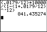
Suppose you want to borrow $10,000 for an automobile. Navy Federal Credit Union offers a loan at an annual rate of 1.79% amortized over 12 months. The payment would be
Since payments are made to the penny, a payment of $841.44 would lead to an overpayment of almost a half of a penny. While this may not seem like much, over the term of the loan it can add up. Financial institutions need to accurately account for these small amounts to insure their books are balanced. An amortization table helps them to do this.
Amortization tables generally have five columns. These columns track the payment number, the amount of the payment, the interest paid in the payment, the portion of the payment applied to the balance, and the outstanding balance on the loan after the payment is made. Let’s look at how the amounts in the table are calculated. We’ll do this by looking at the different rows of the table, one at a time.
The first row of the table helps us to establish the initial balance on the loan. We call it payment 0 since it does not correspond to an actual payment. Using this balance, we can determine the portion of the payment, $841.44, that is applied to the balance and the portion that is interest.
The interest in the payment is calculate by multiplying the interest rate per period times the balance at the end of the previous period,
Interest in Payment 1 = 0.0179/12 · $10,000 ≈ $14.92
In this amortization table, we will round interest amounts to the nearest penny. In practice, you should check with the lender to see how they round interest in the table.
Since the amount applied to balance is the difference between the payment and the interest,
Amount in Payment 1 Applied to Balance = $841.44 – $14.92 = $826.52
This amount reduces the balance at the end of the period,
Balance at the End of the First Period = $10,000 – $826.52 = $9173.48
This strategy is also used to fill in the amounts for the second payment. However, in this case, the interest is calculated using the balance after the previous period.
As the balance decreases, the interest also decreases. This means that a larger and larger portion of the payment goes to paying off the balance.
Payments 3 through 11 are carried out in a similar fashion to give the next few rows. Remember, in this table we are rounding interest amounts to the nearest penny.
For the last payment, we need to pay off the outstanding balance of $840.11. This means the amount of the last payment applied to the balance must be $840.11. The interest in the last payment is
Interest in Payment 12 = 0.0179/12 · $840.11 ≈ $1.25
Combining these two amounts gives the amount of the last payment,
Amount of Payment 12 = $840.11 + $1.25 = $841.36
With these amounts, we can complete the amortization table.
If we add the interest amounts, we find the total amount of interest paid is $97.20.
If we round the payment or interest amounts differently, the amortization table yields different amounts of interest. In the next example, we round all payments and interest amounts up to the nearest penny to see how these change the total amount of interest paid.
Example 4 Make an Amortization Table
Suppose Navy Federal Credit Union rounds all interest and payment amounts up.
a. Find the amortization table on a loan of $10,000 amortized at an annual rate of 1.79% over 12 months with monthly payments.
Solution The terms of the loan are the same as was described above. If the payment is rounded up, we still get a payment of $841.44. When we carry out the process described earlier, we get the table below.
In this table, several of the payments include a slightly higher amount of interest. This means that less of the payment goes towards the outstanding balance. This amount is made up in the last payment where $840.19 is paid to bring the balance to zero. This causes the final payment to be slightly higher.
b. Add the interest amount in the third column to find the total amount of interest paid.
Solution The sum of the interest amounts is $97.29. This is slightly higher than when interest amounts are rounded to the nearest penny. This is to be expected since we rounded all interest amounts up.
The payments and interest amounts may be rounded to the nearest penny, rounded up to the nearest penny, or rounded down to the nearest penny. In all cases, any discrepancies are made up in the final payment.