Many factors influence the output from a business. The quality and quantity of a particular type of technology might inhibit or enhance the output of a business. A company making leather wallets by hand will produce many fewer wallets in a given amount of time compared to a company that uses stitching and cutting machines to make the wallets. Similarly, utilizing more laborers allows a company to divide the tasks required for production among the employees so that each employee is able to specialize in a particular aspect of the production process. Such specialization allows the laborers to work more efficiently resulting in higher rates of production. However, too many employees results in overcrowding and eventually causes the output to increase at a lower rate. This pattern of production is the result of the Law of Diminishing Returns.
Law of Diminishing Returns
When an input is increased, such as labor, while all others are held constant, the resulting increase in production will become larger and larger until the point of diminishing returns. After the point of diminishing returns, the increase in production becomes smaller and smaller.
Since the Law of Diminishing Returns refers to changes in production as an input to production is changed, you would expect that we would be able to relate the derivative of the production function, marginal production, to the point of diminishing returns.
The top graph in Figure 7 shows a typical production function in which all inputs except one, like labor, are held constant. As the input is increased, the output increases at a greater and greater rate until the point of diminishing returns. After the point of diminishing returns, the output continues to increase but at a smaller and smaller rate.
The bottom graph in Figure 7 shows the derivative of the production function, marginal production. Since the point of diminishing returns occurs at the steepest point on the production function, the corresponding input on the derivative of the production occurs at a relative maximum.
To find this relative maximum, we need to find a critical value on the second derivative.
Figure 7 – (a) The production function
and (b) its first derivative.
The bottom graph in Figure 8 shows the second derivative of the production function. The critical value of the first derivative occurs where the second derivative is zero. The second derivative is positive on the left side of the point of diminishing returns and negative on the right side. This indicates that the derivative of the production function changes from increasing to decreasing. It also shows that the production function changes from concave up to concave down and has a point of inflection. So the point of diminishing returns on the production function is a point of inflection. We can use this fact to find the point of diminishing returns.
Figure 8 – (a) The production function
and (b) its second derivative.
Example 9 Find the Point of Diminishing Returns
If we assume labor is the only input to production that can be varied, the relationship between the number of barrels of beer Q (in millions) produced at the Boston Beer Company and the number of employees L (in thousands) from 2000 to 2007 is
Find the point of diminishing returns.
Solution The point of diminishing returns is obtained from the second derivative, by finding the point of inflection. The first derivative is easily calculated:
The second derivative is calculated by taking the derivative of the first derivative,
The point of diminishing returns occurs where the production function changes from concave up to concave down. For a continuous function like this one, this occurs when the second derivative changes from positive to negative. Set the second derivative equal to zero and solve for L to find where the concavity might change:
For this value to correspond to a point of diminishing returns, the function must change from concave up to concave down at this value. Test a value on either side of L ≈ 0.365 in the second derivative to yield the number line:
On the left side of L ≈ 0.365, the second derivative is positive so the function is concave up. The concavity changes on the right side of L ≈ 0.365 since the second derivative is negative in that interval.
This value is a point of diminishing returns and the number of barrels when the number of employees is 365 is
What does the second derivative of a function tell you about a function?
The first derivative of a function tells us the rate at which a function changes. If the first derivative is positive over some interval, then the values on the function are increasing as we move left to right over the interval. If the first derivative is negative over some interval, then the values on the function are decreasing as we move left to right over the interval.
The relationship between a function and its derivative is always the same. The derivative tells you whether the function it comes from is increasing or decreasing. If the function we are examining is the first derivative itself, the second derivative tells you whether the first derivative is increasing or decreasing. The curvature of the graph of a function is influenced by whether the first derivative is increasing or decreasing.
A graph is concave up over an interval [a, b] if the graph is above its tangent lines at each point in the interval.
A graph is concave down over an interval [a, b] if the graph is below its tangent lines at each point in the interval.
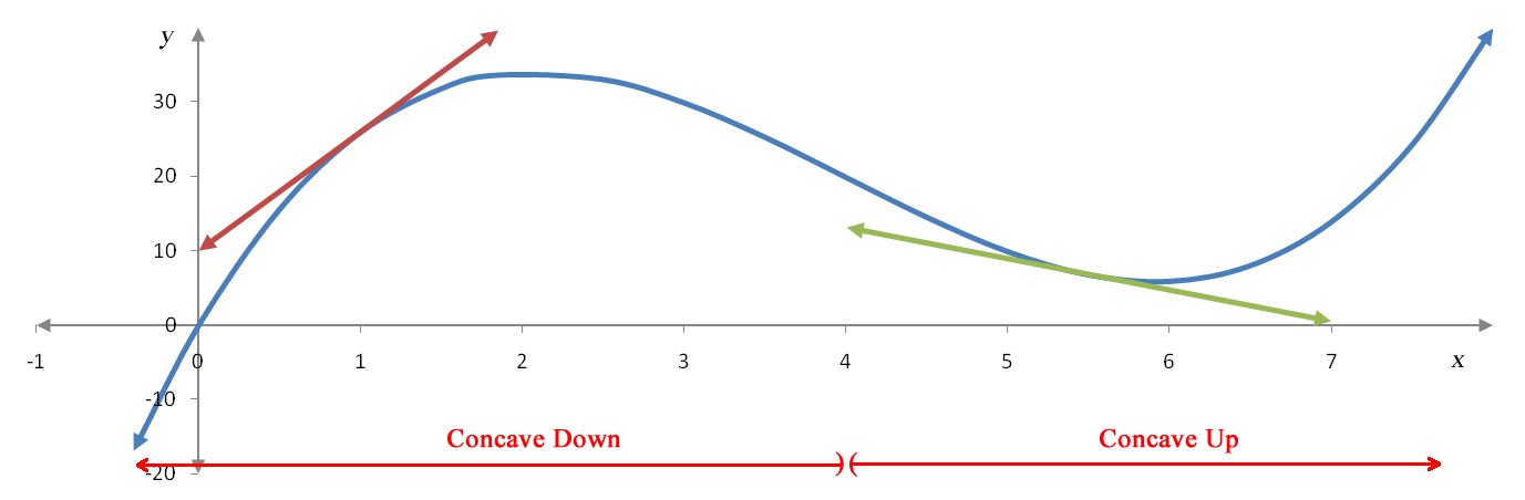
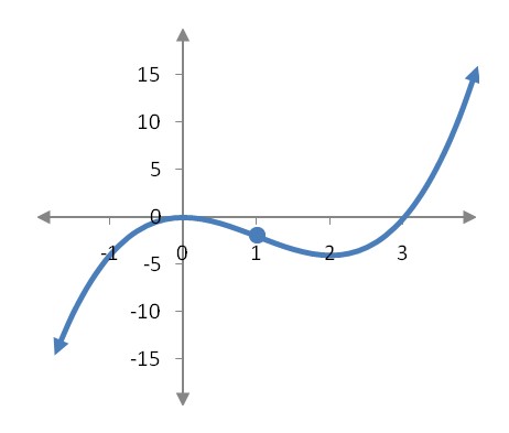
Let’s examine a specific function, f (x) = x3 – 12x2 + 37x, to see how the concavity of a graph is related to the second derivative of f (x).
Figure 2 – A graph of y = f (x) with two tangent lines.
In Figure 2, any point on the graph to the left of x = 4 such as the point at x = 1 is below its tangent line so the graph is concave down over the interval (-∞, 4). Any points to the right of x = 4, such as x = 5.5, are above the corresponding tangent line so the graph is concave up over the interval (4, ∞). Informally, the graph bends downward when the graph is concave down and bends upward when the graph is concave up.
The function’s values locate the heights of the points on the graph. Over the x values listed in the table, all y values are positive so the function is graphed above the x axis at those x values.
The first derivative values indicate where the function is increasing or decreasing. When the first derivative is positive, the function’s graph is increasing. When the first derivative is negative, the function’s graph is decreasing.
The values of the second derivative indicate where the function’s graph is concave up or concave down. When the second derivative is negative, the function’s graph is concave down. When the second derivative is positive, the function’s graph is concave up.
We can understand this behavior by examining how the first derivative is changing in the table.
To the left of x = 4, the first derivative values change from 16 to -8. Since the first derivative values are decreasing, the derivative of the first derivative, the second derivative, must be negative to the left of x = 4.
To the right of x = 4, the first derivative values change from -8 to 16. Since the first derivative values are increasing, the second derivative, must be positive to the left of x = 4.
Concavity and the Second Derivative
When the graph of a function f (x) is concave up, the second derivative f ″(x) is positive.
When the graph of a function f (x) is concave down, the second derivative f ″(x) is negative.
The points on the function where the function changes concavity, concave down to concave up or concave up to concave down, are called points of inflection. We can use a process, similar to how we tracked the sign of the first derivative, to track the sign of the second derivative. This process allows us to determine where a function’s graph is concave up or concave down and the location of any inflection points.
Example 6 Determine Concavity
Let f (x) be the function defined by
a. Where is the function f (x) concave up?
Solution The concavity of a function can be determined from the second derivative of a function. For this function, the first derivative is
and the second derivative is
The function f (x) is concave up when the second derivative is positive. We can use a number line, in a manner similar to how we tracked the sign of the first derivative, to track the behavior of the second derivative. Start by locating where the second derivative f ″(x) is equal to zero or undefined:
There are no values where the second derivative is undefined. This x value is where the second derivative could potentially change sign. By testing the second derivative on either side of x = 1, we can decide where the second derivative is positive and where it is negative.
Start the second derivative number line by labeling x = 1 on it with the behavior of the second derivative above that label.
Test x = 0 and x = 2 in the second derivative so that we can label the corresponding signs on the number line.
We can add this information to the number line.
Since the second derivative is positive on the right side of x = 1, the function is concave up on the interval [1, ∞).
b. Where is the point of inflection on the function f (x)?
Solution The number line from part a indicates that the concavity changes from down to up at x = 1. The corresponding y value is calculated from the original function,
This point, (1, -2) , is the point of inflection.
Figure 3 – The point of inflection at (1, -2) is where the concavity of the function changes.
Example 7 Find the Point of Inflection
Companies like Apple spend money on research and development to help them develop new products. Products like Ipods, Iphones and Ipads all started with an investment in research and development and now are a large portion of Apple’s sales. From 2001 through 2010, sales S(R) (in billions of dollars) are related to research and development expenditures R (in billions of dollars) via the function
(Source:Modeled from Apple Annual Reports)
a. Find the point of inflection.
Solution To find the point of inflection, we must find any points where S″(R) is equal to zero or undefined. Once we have located these points, we can test the second derivative on either side of these values to see if the concavity changes.
The first derivative of S(R) is
By taking another derivative of the first derivative, we get the second derivative
The second derivative is always defined, so the only values where the concavity might change correspond to S″(R):
This value is approximately equal to 1.058 billion dollars of research and development expenditures. The concavity may or may not change at this value of R. To check the concavity on either side of R ≈ 1.058, make a number line for reasonable values of research and development expenditures. Test the second derivative on either side of the potential point of inflection.
The function S(R) is concave down on the left side of R ≈ 1.058 and concave up on the right side of R ≈ 1.058. Since the concavity changes, this value corresponds to a point of inflection. The point is located on the graph by substituting 1.058 in the original function,
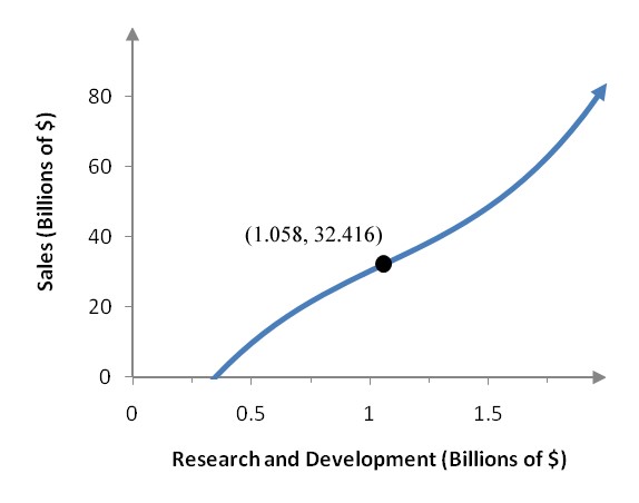
This point, (1.058, 32.426), is also the location of the point of inflection.
b. What does the point of inflection tell you about the relationship between sales and research and development expenditures?
Solution Let’s examine the graph of the sales function S(R).
Figure 4 – The sales at Apple as a function of research and development spending.
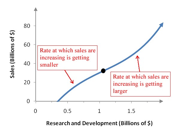
This function is increasing throughout its domain indicating that as research and development increases, sales increase. When research and development spending less than 1.058 billion dollars, increasing spending leads to higher sales but at a reduced rate. This is because the slope of the sales function is getting smaller as we increase R in the interval [0, 1.058). Once research and development spending is greater than 1.058 billion, increased spending leads to greater and greater sales. This is because the slope of the sales function is getting higher as we increase R in the interval (1.058, ∞).
Figure 5 – Increasing research and development spending beyond 1.058 billion dollars leads to greater and greater sales.
Example 8 Find the Point of Inflection
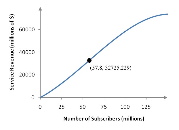
Wireless companies like Verizon Wireless are able to increase their revenue by adding more subscribers. However, as the number of subscribers is increased, the amount charged often decreases to attract customers from competing wireless companies. For the years 2004 through 2009, the service revenue R(S) (in millions of dollars) as a function of the number of subscribers S (in millions of subscribers) can be modeled by the function
(Source: Modeled from data in Verizon Annual Reports)
Find the point of inflection.
Solution To find the point of inflection, we need to calculate the first derivative,
and the second derivative,
The graph might change concavity where the second derivative is equal to zero or undefined. Since the second derivative is a linear function, it is defined everywhere. Set the second derivative equal to zero and solve for S to find where R″(S):
The fraction is approximately 57.8. Let’s make a number line for the second derivative R″(S) and track the sign of the second derivative on the interval [0, ∞). Two useful second derivative values are
Label these values on a second derivative number line.
The service revenue function is concave up for values less than 57.8 million subscribers and concave down for values greater than 57.8 million subscribers. The service revenue at this number of subscribers is
Figure 6 – A graph of R(S) with the point of inflection.
When the number of subscribers is less than 57.8 million, adding subscribers leads to more and more revenue since the slope of the function is getting larger. However, once 57.8 million subscribers is exceeded, the service revenue continues to increase but at a smaller and smaller rate since the graph gets less steep. The point of inflection is the dividing line between where the rate of change of service revenue gets larger and larger or smaller and smaller.
The second derivative is an example of a higher derivative. By taking the derivative of the second derivative, we obtain another higher derivative, the third derivative. The notation for the third derivative follows the pattern established by the second derivative.
Any of the following notations may be used to write the third derivative of a function y = f (x):
By taking the derivative of another derivative, we may calculate other higher derivatives. These higher derivatives may be written in a similar manner. For derivatives higher than the third derivative, we write the nth derivative as f(n)(x).
For the function f (x) = 5x4 – 7x2 + 2x – 1, the first and second derivatives were calculated earlier as
The derivative of the second derivative, the third derivative, is calculated by taking the derivative of the second derivative. We can continue to take the derivative of the derivative to obtain higher derivatives:
Since the derivative of a constant is zero, the fifth derivative and those higher are equal to zero.
Example 4 Calculate the Fourth Derivative
Let
Find the fourth derivative h(4) (x).
Solution The first derivative is
We can follow the same strategy to get the second derivative,
the third derivative,
and the fourth derivative,
Example 5 Calculate the Third Derivative
LetFind the third derivative
Solution To find the first derivative, use the Product Rule for Derivatives with the factors and corresponding derivatives,
The product rule leads to
The second derivative is simply the derivative of the first derivative or
Rewrite as t -1 to make the next derivative easy to do. The third derivative is
The third derivative is rewritten with a positive exponent as .
The second derivative is the derivative of the derivative. To help identify this process, the first time we take a derivative of a function we call it the first derivative. The first derivative, as we have seen earlier, is symbolized in several different ways. If we take the first derivative of a function y = f (x), the first derivative is written as
Several notations for the second derivative are used.
Any of the following notations may be used to write the second derivative of a function :
We can take the derivative of the first derivative by applying the rules for derivatives to the first derivative. If f (x) = 5x4 – 7x2 +2x – 1, then we can apply the Sum / Difference, Product with a Constant, and Power Rules for Derivatives to yield the first derivative
If we use these rules again on the first derivative, we get the second derivative,
The process for finding the derivative is the same as we have used in Chapter 11. The only difference is the starting point. When finding the first derivative of a function, we take the derivative of the function. For the second derivative, we take the derivative of the first derivative.
Example 1 Calculate the Second Derivative
Let f (x) = x3 -4x2 + 6x +12. Find the second derivative f ″(x).
Solution The first derivative of is found by applying rules for derivatives,
To find f ″(x), take the derivative of f ′(x) = 3x2 – 8x +6:
The second derivative is f ″(x) = 6x – 8.
Example 2 Calculate the Second Derivative
Let
Find the second derivative
Solution The first derivative is found with the Product Rule for Derivatives using the factors
The first derivative is
Apply the product rule again to find the second derivative with the factors
The second derivative is
The second derivative is
Example 3 Calculate the Second Derivative
Let Find the second derivative g″(x).
Solution Use the Quotient Rule for Derivatives to find the first derivative with
The first derivative is
To compute the second derivative, take the derivative of the first derivative with the Quotient Rule for Derivatives,
The second derivative is
The second derivative expression can be simplified further by factoring the numerator:
Earlier in this chapter, we used definite integrals to find the area under a function and above the x axis. By writing
or
we find the area under the function, above the x axis, and between x = a and x = b. In this section, we’ll use these areas to find the area between f (x) and g(x) from x = a to x = b.
We’ll use this area to define two important concepts in economics, consumers’ surplus and producers’ surplus.

 The top graph in Figure 7 shows a typical production function in which all inputs except one, like labor, are held constant. As the input is increased, the output increases at a greater and greater rate until the point of diminishing returns. After the point of diminishing returns, the output continues to increase but at a smaller and smaller rate.
 The bottom graph in Figure 8 shows the second derivative of the production function. The critical value of the first derivative occurs where the second derivative is zero. The second derivative is positive on the left side of the point of diminishing returns and negative on the right side. This indicates that the derivative of the production function changes from increasing to decreasing. It also shows that the production function changes from concave up to concave down and has a point of inflection. So the point of diminishing returns on the production function is a point of inflection. We can use this fact to find the point of diminishing returns.