In section 11.2, we introduced the idea of the instantaneous rate of change of a function. This idea is critical to understanding how a quantity is changing with respect to another. The instantaneous rate of change of a function f (x) with respect to x at is also called the derivative off (x) at x = a.
The derivative of f (x) at x = a is defined as
provided the limit exists. The symbol f ′(a), is read “f prime of a”.
In this section we’ll look at the derivative of a function from a geometric viewpoint by examining slopes of secant lines and how they can be used to find the slope of a tangent line. We will also find the derivative of a function at a point. This is essentially the same process we used to calculate the instantaneous rate of change of a function given by a formula at a point.
Once we have looked at the idea of a derivative geometrically and have taken the derivative of several functions, we will explore what a derivative of a function tells us for several business functions.
The average rate of change is useful for calculating how quantities change with respect to each other. It allows us to quantify these changes and to understand whether one quantity is increasing or decreasing with respect to another quantity. Unfortunately, the average rate of change has its limitations. These limitations can be illuminated by calculating the average rate of change of the Dow Jones Industrial Average on May 6, 2010 with respect to time. The Dow Jones Industrial Average (DJIA) is an index that tracks 30 large companies on the New York Stock Exchange (NYSE). On this date, the stock market was preoccupied with news of a debt crisis in Greece. The NYSE opened at 9:30AM and the Dow Jones Industrial Average was at a level of 10862.22 points. It closed at 4:00PM at a level of 10520.32 points.
Let’s look at how the Dow Jones Industrial Average changed that day by calculating its average rate of change with respect to time. To find this rate, we must calculate the change in the index that day, ΔDJIA, and the change in time that the NYSE was open for trading, Δt.
The change in the index is calculated by subtracting the opening level of the index from the closing level of the index,
In the language of the stock exchange, the Dow Jones Industrial Average lost 341.9 points on May 6, 2010.
Since the NYSE is open from 9:30AM to 4:00PM, the change in time is 6 ½ hours or 390 minutes. We could use hours or minutes to calculate the average rate of change, but in this case we’ll use minutes and set Δt = 390.
Using these changes, we can calculate the average rate of change,
This means that, on average, the Dow Jones Industrial Index dropped slightly less than one point for each minute the NYSE is open on May 6, 2010. This may not seem like much, but in general the Dow Jones Industrial Average changes very little from day to day.
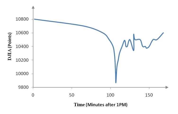
On May 6, 2010, the Dow Jones Industrial Average suffered a flash crash. A flash crash occurs when the index drops a large amount over a very short period of time. During the flash crash on May 6, 2010, the DJIA dropped over 900 points in a matter of minutes. Shortly after this drop, the index recovered these losses.
Figure 1 – This graph shows the steep drop in the DJIA before recovering on May 6, 2010.
The average rate of change we found earlier was calculated over the span of the entire trading day or 390 minutes. It takes into account the opening and closing levels of the Dow Jones Industrial Average, but nothing else over the course of the trading day. It shows what happen, on average, during the day, but not what happen in a ten minute period around 2:45PM.
To calculate how fast the DJIA was dropping during the flash crash, we need to calculate the instantaneous rate of change of the Dow Jones Industrial Average with respect to time. Like the average rate of change, the instantaneous rate of change measures fast two quantities are changing with respect to each other. As the term “instantaneous” indicates, the instantaneous rate of change measures how fast one quantity changes when another quantity changes by a very small amount.
In the case of the Dow Jones Industrial Average, we would like to calculate the instantaneous rate of change of the with respect to time at the height of the flash crash. We’ll do this by calculating how much the index changes over a very short period of time. This will tells us how fast the Dow Jones Industrial Average was dropping at the instant the flash crash occurred.
In this section, we’ll examine how quantities change with respect to each other. This is a topic that is not entirely unfamiliar. On a long trip in a car, you may be interested in knowing how the distance traveled changes with respect to how much time has elapsed. By knowing how many miles per hour your vehicle has averaged, you get an idea of how long it will take you to arrive at your destination.
Auto manufacturers are also interested in how far a vehicle will travel, but as the amount of gasoline that is in the tank changes. By comparing the distance traveled to the amount of gasoline consumed, they get an idea of how efficient the vehicle is. Vehicles that achieve a higher miles per gallon are more efficient than those that achieve a lower miles per gallon.
An insurance analyst might be interested in knowing how the percentage of people who are driving uninsured varies as the percentage of people who are unemployed changes. By understanding how these percentages vary with respect to each other, they can better understand the risk of being in an accident with a person who is uninsured.
Among citizens, taxes are a contentious issue. Every person has their own opinion regarding how much they should be taxed or what parts of their income should be taxed. Above all, people feel that taxes should be fair. Taxes help to fund the various functions we expect from the federal government.
In the United States and many other countries, the tax rate increases as taxable income rises. In many states, a similar state income tax exists. In the state of Arizona (2011), several tax brackets exist for individuals with corresponding tax rates.
This table reflects the progressive side of the tax. The more you make, the higher the tax rate is. However, many people get squeamish when they change income brackets. If your taxable income increased the following year from $9,999 to $10,001, would the change in tax rates lead to a jump in the amount you paid?
In this section, we’ll examine this question in the context of continuous functions. We’ll learn how to recognize a continuous function. This will help us to determine if there are any jumps in the amount a person pays in Arizona when an income increase moves them from one tax bracket to another.
The limits in sections 10.1 and 10.2 were limits in which the value of x approached some finite value. By writing
we were looking for the behavior of the function f (x) as x got closer and closer to the value a. In this section we’ll learn how to evaluate a second type of limit. In limits at infinity, we look at the behavior of the function as x gets more and more positive or as x gets more and more negative. We symbolize limits like this by writing
or
As with other limits, we may evaluate the limit with a table, graph, or using algebra.