The constants and coefficients in a linear programming problem are usually estimates. As estimates, the values of the constants and coefficients may change as new information is developed or business conditions change. Sensitivity analysis helps us to evaluate how an optimal solution may change if these estimates change.
The Simplex Method and the Standard Minimization Problem
In Section 4.3, the Simplex Method was used to solve the standard maximization problem. With some modifications, it can also be used to solve the standard minimization problem. These problems share characteristics and are called the dual of the other. In this section, we learn what a standard minimization problem is and how it is connected to the standard maximization problem. Utilizing the connection between the dual problems, we will solve the standard minimization problem with the Simplex Method.
The Simplex Method and the Standard Maximization Problem
In Section 4.2, we examined several linear programming problems. The common theme to these problems is the number of decision variables. To be able to solve these linear programming problems graphically, they must have exactly two decision variables.
In this section you will learn how to solve linear programming problems with two or more decision variables. This strategy, called the Simplex Method, will allow us to solve the problems from section 4.2 as well as other maximization problems with more than 2 variables. Since large numbers of decision variables are common in business and industry, the Simplex Method and similar variations are standard tools used to analyze linear optimization problems with hundreds of decision variables and hundreds of constraints.
Systems of inequalities constrain the values of the variables that are reasonable for a problem. For example, in the craft brewery problem in Section 4.1, the system of inequalities defined a region on a graph that told us how many barrels of pale ale and porter that could be produced. The ordered pairs on the graph insured that the brewery does not exceed monthly production or exceed their ability to ship, store, and process malt and hops.
Figure 1 – The shaded area of the graph represents possible solutions to the system of inequalities for the craft brewery.
There are an infinite number of combinations on the graph that make all of the inequalities in the system true at the same time. Which of these solutions is the best for the brewery to produce? How do we pick out the optimal production level for each type of beer? These questions can be solved by posing a linear programming problem. By solving the linear programming problem, we find the production level for beer that meets some criteria and satisfies the constraints given by the system of inequalities.
In Chapter 2, we were concerned with systems of linear equations. In this section, we’ll change the equal signs in systems of linear equations to inequalities to yield systems of linear inequalities. Systems of linear inequalities occur frequently in business where production is constrained by the availability of materials, labor, or transportation.
For instance, over the last twenty years craft beer has become very popular. One of the largest craft breweries produces five different beers throughout the year. The monthly capacity of the brewery is 50,000 barrels of beer (one barrel is 31 gallons). If x1 through x5 represent the monthly production of each of the different types of beer in barrels, we can writeThe sum of the variables represents the total monthly production, so setting this sum equal to 50,000 tells us the brewery is operating at its monthly capacity of 50,000 barrels.
However, the brewery may not operate at its full capacity. If the brewery is producing less than 50,000 barrels of beer, we would write
The inequality points to the smaller quantity so the expression on the left, the total monthly production, is smaller than 50,000 barrels. If the brewery is operating above capacity, the inequality
indicates the total monthly production is greater than 50,000 barrels. Inequalities with < or > are called strict inequalities.
Inequalities may also involve a combination of <, >, and =. By writing
we know that the brewery is operating at or below capacity. We would read this as the total monthly production, x1 + x2 + x3 + x4 + x5, is less than or equal to 50,000. If the inequality is reversed,
we say that the total monthly production is greater than or equal to 50,000 barrels.
In this section, we’ll examine solutions of inequalities involving two variables. When only two variables are involved, we can graph the solutions on a rectangular coordinate system and shade the region of the graph where the ordered pairs satisfy the inequality. The ordered pairs satisfying the inequality result in a true statement when they are substituted into the inequality.
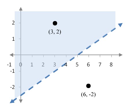
Let’s check to see if the ordered pair (x, y) = (3, 2) satisfies the inequality x – 2y < 5. By setting and in the inequality, we get the statement
3 – 2(2) < 5
The left side of the inequality is equal to -1. This value is less than 5 so the inequality is true and the ordered pair satisfies the inequality. The ordered pair (x, y) = (6, -2) does not satisfy the inequality x – 2y < 5 since
6 – 2(2) < 5
is not a true statement.
In a graph of the inequality , all ordered pairs satisfying the inequality lie in the shaded region in Figure 2. Ordered pairs that do not satisfy the inequality lie in the unshaded region or on the dashed border of the shaded region.
Figure 2 – All ordered in the shaded region satisfy the inequality x – 2y < 5. Ordered pairs on the dashed line like (5, 0) do not satisfy the inequality x – 2y < 5.


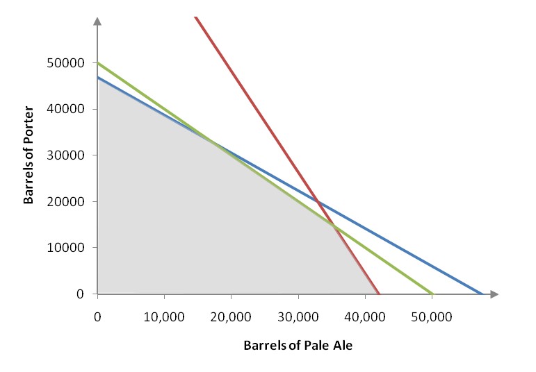
 Figure 1 – A copper brewing kettle at a craft brewery.