Category: Applied Calculus Ebook

What is a function?

A variable is a symbol that represents a quantity that may vary. Typically a variable is a letter of the alphabet. However, not all letters of the alphabet are necessarily variables. For instance, in physics the letter c is a constant that represents the speed of light. It is called a constant because the speed of light in a vacuum does not change. Letters in other alphabets such as the Greek alphabet can also be variables or constants. The letter π (pronounced pi) is a constant used in geometry that has a value that is approximately 3.14157.

Mathematics allows us to describe relationships between quantities in a variety of ways. In your mathematical experience, you have probably been exposed to formulas that relate variables like x and y. There is nothing special about the letters x and y. We could have used any letters in a formula. However, most algebra classes use the variables x and y so we’ll start there and introduce other variables later that are appropriate in finite mathematics.
A very simple formula that relates the variables x and y is

y = 2x

Since this formula is solved for y, you might think of substituting a number in place of x to obtain a value for y. For instance, a value of x = 3 corresponds to a value of y = 6,

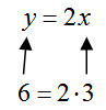
We think of this as inputting the value of x = 3 to obtain an output of y = 6. The variable corresponding to the input, x, is called the independent variable. The variable corresponding to the output, y, is the dependent variable. We use the term dependent to emphasize the fact that the value for y depends on the input x. There is nothing special about the letters used in the relationship or even which letter matches with the independent or dependent variables. These terms are used to help describe the input and output from a relationship between two variables. Consider the formula

Since this formula is solved for x, we would use it to take a value for y to compute a value for x. In this case we would think of y as the independent variable and x as the dependent variable. This means that an input of y = 6 corresponds to an output of x = 3. These are the exact same values as y = 2x. The reason for this is that it can be solved for x to give :

Whether we start with x and multiply by 2 to get y or start with y and divide by 2 to get x, the relationship between x and y is the same. The only change is our perspective on the independent and dependent variable. In each of these cases, the variable that is solved for is the dependent variable.

The picture gets murkier if the equation is not solved for a variable. Suppose we have the equation

y – 2x = 0

This equation is not solved for x or y. It is not clear whether x or y is the independent variable. In a case like this, we can specify which variable is the independent variable. The choice we make may reflect the quantity the variable represents or may simply be our own personal choice.

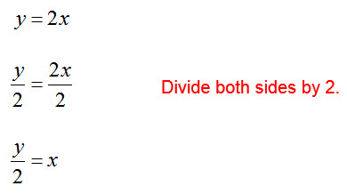
If we decide to make the independent variable x, we need to solve the equation for y to yield

y = 2x

In this form, it is easy to input a value for x to calculate an output y. If we decide to make the independent variable y, we need to solve the equation for x to yield

If we have a value for y, this equation can be used to calculate an output x. The variable chosen for the independent variable is often up to the user. In other contexts the independent variable is determined by the traditional choice made by practitioners in the field.

Example 1     Write an Equation with a Specified Independent Variable

Suppose you have the equation 10P + 2Q = 100 relating the quantity Q of a product demanded by consumers and the price P in dollars.

a. Write the equation with P as the independent variable.

Solution To write 10P + 2Q = 100 with a certain variable as the independent variable, solve the equation for the other variable. If P is to be the independent variable, solve the equation for Q:

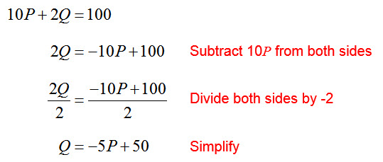
b. Write the equation with Q as the independent variable.

Solution If Q is to be the independent variable, solve the equation for P:

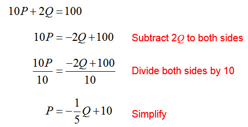
Economists traditionally choose the quantity Q to be the independent variable when working with functions relating price and quantity. In this format, we can see that as the quantity Q demand by consumers increases, the price of the good must decrease to make it attractive to the consumer.

---

The term function describes a special type of relationship between the independent and dependent variable. These values for these variables are chosen from two sets called the domain and range of the function. The values for the independent variable are chosen from the domain and the values for the dependent variable are chosen from the range.

The phrase “a function of” is used to tell the user what the independent variable is. For instance, the phrase “y as a function of x” indicates that the independent variable is x and the dependent variable is y.

To determine if an equation describes a function, identify the independent and dependent variable. Then determine if each value of the independent variable selected from the domain of the correspondence matches with no more than one value of the dependent variable. If there is no more than one match, then the correspondence is a function.

Example 2     Determine If An Equation Represents a Function

Does the equation 10P + Q = 500 describe P as a function of Q?

Solution Since this example specifies P as a function of Q, we know that the independent variable is Q and the dependent variable is P. To make it easier to see how P and Q are linked, solve the equation for the dependent variable P:

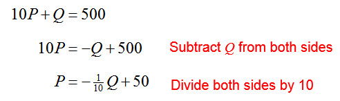
In this form, we can see that a value like Q = 100 corresponds to one value of P, P = 40. In fact, for any value of Q you get only one value P. This means that this equation describes a function.

---

Example 3     Determine If An Equation Represents a Function

Does the equation x² + y² = 4 describe y as a function of x?

Solution This example specifies y as a function of x so we know that the independent variable is x and the dependent variable is y. Like the previous example, solve for the dependent variable y:

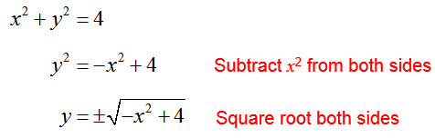
If we try a value like x = 10, the radicand becomes -10² + 4 or -96. Assuming we are using real numbers, we can’t take the square root of a negative number. The input to this equation is not a reasonable input because it is not a part of the domain of this function.

To be a part of the domain of this function, the input to this function needs to make the radicand nonnegative. The value of x must satisfy –x² + 4 > 0. Inspecting this inequality, we can see that –x² + 4 = 0 at x = -2 or 2. Values between -2 and 2 like x = 0 make the expression positive. This means the domain of this relationship is all real numbers greater than or equal to -2, but less than or equal to 2.

If we pick values from the domain like x = 0, we get two outputs, or . Since there is a number in the domain that corresponds to more than one member of the range, the relationship x² + y² = 4 does not describe a function.

A graph of this equation verifies this conclusion. The graph of this equation is a circle.

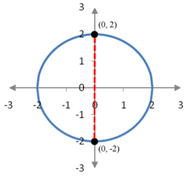
Figure 1 – For this graph, any input between x = -2 and x = 2 leads to two outputs. This means the graph does not correspond to a function.

On this circle, we can see that the line x = 0 crosses the graph at the points (0, 2) and (0, -2). This means that the input x = 0 corresponds to two different outputs. In fact, any input except for x = 2 or x = -2 corresponds to two outputs since vertical lines cross the graph in two places.

---

In Example 2, we found that by writing 10P + Q = 500 in the form  we could easily check to see if each value of Q led to no more than one value of P. This told us that this relationship was a function since each value of the independent variable led to no more than one value of the dependent variable. Now let’s look at this function a little closer.

You may have thought that the variables P and Q were a bit strange. After all, in most math textbooks you typically work with the variables x and y. In these situations you were working with equations and their corresponding graphs in the x–y plane. You were most concerned with the shapes of these graphs and the equations usually had little basis in an application.

In business and finance, every equation is based on an application. The names of the variables often help you to understand what they represent. For instance, the variables P and Q usually represent the price and quantity of some good. These variables can be related to each other in one of two different ways. A demand function relates the price P of a good to the quantity Q of the good demanded by consumers. The function

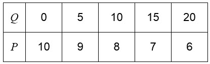
is an example of a typical demand function. As Q gets larger, bigger and bigger negative numbers are added to 50 resulting in smaller and smaller values. A graph of this function reflects this characteristic. In Figure 2, the graph is a line that drops as you move from left to right. This means that as the quantity is increased (move left to right), the price drops.

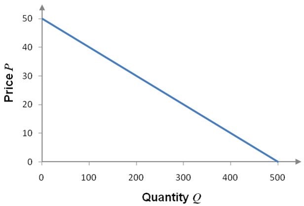
Figure 2 -As the quantity Q increases from 0 to 500 horizontally, the price P drops from 50 to 0. This means that the quantity demanded by consumers increases as the price drops.

This function’s graph is a straight line. A function whose graph is a straight line is called a linear function.

Looking at the graph, it is easy to recognize a linear function. We would also like to be able to recognize a linear function from its equation.

It is easy to read this definition without examining how it applies to the line . The equations y = mx + b and may look different, but are really very similar.

The definition for a linear function contains four letters: y, m, x, and b. Some of these letters are variables and others are constants. To ensure that the user of this function knows which letters are variables and which letters are constants, we need to define the variables.

One way of doing this is to write, y is a linear function of x. By writing this phrase, we know that the variables in the equation y = mx + b are x and y. All other letters are constants representing numbers.

By modifying the phrase, we can write other linear functions with different variables. The phrase “P is a linear function of Q” corresponds to the equation

P = mQ + b

where Q is the independent variable, P is the dependent variable and m and b are constants. An example of a linear function in which P is written as a linear function of Q is

In this case, the value of m is –¹/₁₀ and b is 50.

Example 4     Does An Equation Correspond to a Linear Function?

Decide if the equation 5P + 10Q = 100 can be written so that P is a linear function of Q.

Solution To decide if the equation can be written so that P is a linear function of Q, we need to rewrite the equation in the form P = mQ + b. By stating “linear function of Q”, the example implies that the variable on the right side is Q. Solve the equation for P to put the equation in this form:

The equation can be written in the proper form with m = -2 and  b = 20.

---

Example 5     Does An Equation Correspond to a Linear Function?

Decide if the equation 5P + 10Q = 100 can be written so that Q is a linear function of P.

Solution Compared to Example 4, this example reverses the role of the variables. “Q is a linear function of P” means that we want to rewrite the equation in the form Q = mP + b. To accomplish this task, we must solve the equation for Q:

The equation can be written in the proper form with m = –¹/₂ and b = 10.

Example 4 and Example 5 suggest that an equation must be solved for the dependent variable to determine if the equation is a linear function. The phrase

Dependent Variable is a linear function of the Independent Variable

allows you to obtain the appropriate form for the linear function. The dependent variable is always written first in this statement and the independent variable is always written after “linear function of”. Based on this phrase, we know the form will be

Dependent Variable = m·Independent Variable + b

An equation that can be written in this form, by solving for the dependent variable, is a linear function. If a function cannot be written in this form, it is not a linear function.

 

How do we make decisions about inventory?

Most businesses keep a stock of goods on hand, called inventory, which they intend to sell or use to produce other goods. Companies with a predictable demand for a good throughout the year are able to meet the demand by having an adequate supply of the good. A large inventory costs money in storage cost and carrying low inventory subjects a business to undesirable shortages called stockouts. A company’s inventory level seeks to balance the storage cost with costs due to shortages.

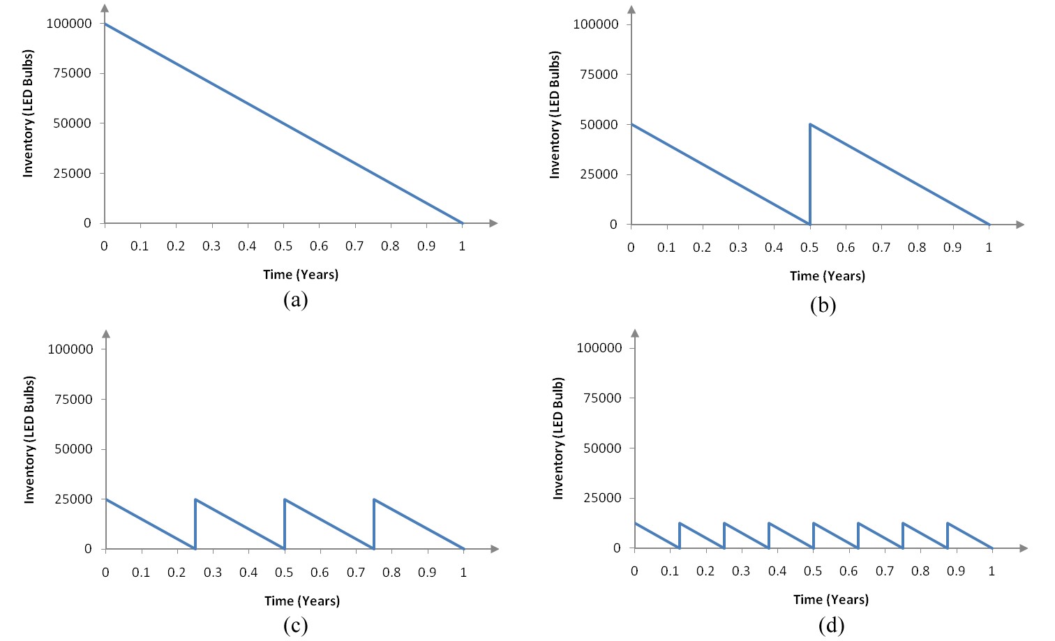
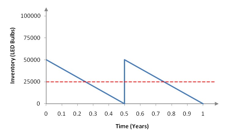
A light emitting diode (LED) is a light source that is used in many lighting applications. In particular, LEDs are used to produce very bright flashlights used by law enforcement, fire rescue squads and sports enthusiasts. Suppose a manufacturer of LED flashlights needs 100,000 LED bulbs annually for their flashlights. The company may manufacture all of the LED bulbs at one time or in smaller batches throughout the year to meet its annual demand. If the manufacturer makes all of the bulbs at one time they will have a supply to make flashlights throughout the year, but will need to store bulbs for use later in the year. On the other hand, if they make bulbs at different times throughout the year, the factory will need to be retooled to make each batch.

Figure 1 – Inventory levels at the manufacturer over a one year period. In (a), all bulbs are made at the beginning of the year and used at a constant rate throughout the year. In (b), two batches of 50,000 are made. In (c), 4 batches of 25,000 are made. In (d), 8 batches of 12,500 are made. In each case, when the inventory reaches 0, the next batch is manufactured instantaneously.

Since the manufacturer does not need to make LED bulbs continuously throughout the year, they will use the manufacturing capacity for other purposes during the rest of the year. When they do manufacture the bulbs, the factory will need to be set up for this purpose. For this manufacturer, it costs 5000 dollars to set up the factory to manufacture LED bulbs. This amount covers all costs involved in setting up the factory such as retooling costs, diminished capacity while the production line is retooled, and labor costs. Each time the company manufactures a batch of bulbs, they incur this cost. Obviously, the more times the plant retools, the higher the total cost is.

The company pays a holding cost to store any LED bulbs not used. The holding cost includes the taxes, insurance, and storage costs that change as the number of units stored changes. If they manufacture all of the bulbs at one time, they will have to store more bulbs throughout the year. For this manufacturing plant, it costs $1 to hold a bulb for one year.

We’ll assume that the company’s production cost does not change throughout the year. In other words, whether they manufacture the bulbs all at once or in several batches throughout the year, it will cost them the same amount per unit to manufacture the bulbs. For this plant, it costs 25 dollars to manufacture an LED bulb.

The total cost for the manufacturer is the sum of the set up, holding and production costs. For other manufacturers, other costs may be included in this sum. However, we’ll assume that the total cost for this plant is restricted to these three costs. If they produce more LED bulbs in each batch, the set up costs will be lower but they will pay a higher holding cost. On the other hand, if they produce fewer bulbs in each batch they will lower the holding cost. This decrease in holding cost is accompanied by an increase in the set up cost since more batches will be needed to meet the annual demand. The manufacturer faces a simple question: how many units should they manufacture in each batch so that their total cost is minimized? The batch size that results in the lowest total cost is called the economic lot size.

Example 3      Find the Economic Lot Size

A manufacturing plant needs to make 100,000 LED bulbs annually. Each bulb costs 25 dollars to make and it costs 5000 dollars to set up the factory to produce the bulbs. It costs the plant 1 dollars to store a bulb for 1 year. How many bulbs should the plant produce in each batch to minimize their total costs?

Solution To find the economic lot size, we need to analyze the costs for the plant and model these costs.

What kind of costs will be incurred? Three different types of costs are described in this example. A set up cost of 5000 dollars is incurred to set up the factory. A production cost of  25 dollars per bulb is incurred for labor, materials, and transportation. Since the demand for bulbs occurs throughout the year, we’ll need to store some of them in a warehouse at a holding cost of 1 dollar per bulb for a year.

Let’s try to solve this naively and simply produce all 100,000 bulbs in one batch. If the demand throughout the year is uniform, we can expect to have an average inventory of

Figure 2 – If all of the LED bulbs are produced in one batch, the average inventory is 50,000 bulbs.

It will cost 1 dollar to store each of these bulbs for holding costs of 50,000 × 1 dollar or 50,000 dollars.  If all of the bulb are produced in one batch, the production line will need to be set up once for a cost of 5000 dollars.To produce 100,000 bulbs at a cost of 25 dollars per bulb will cost 100,000 × 25 dollars or 2,500,000 dollars. The total cost to produce one batch of 100,000 bulbs is the sum of these costs,

The largest cost in this sum is the production cost. If the cost to make a bulb is fixed and we don’t change the number of bulbs produced each year, changing the batch size won’t affect this term.

We can lower the holding cost by producing fewer bulbs in each batch. But this increases the set up cost since the production line will need to be set up more often.

Figure 3 -If the LED bulbs are produced in two batches, the average inventory is reduced to 25,000 bulbs.

If the batch size is reduced to 50,000, the average inventory is reduced to

for storage costs of 25,000 × 1 dollar or 25,000 dollars. The production line will need to be set up twice at a cost of 2 × 5000 dollars or 10,000 dollars.

We will still produce 100,000 bulbs at a cost of 25 dollars per bulb. This will cost 100,000 × 25 dollars or 2,500,000 dollars. The total cost is now

In this case, the holding cost dropped by 25,000 dollars, but the set up cost increased by 500 dollars. This results in a lower total cost.

Continuing with this strategy, we can fill out the following table:

As the lot size decreases, the set up cost increases and the holding cost decreases. Initially, the holding cost is much higher. But for smaller batch sizes, the set up cost is much higher. Somewhere in the middle is a batch size whose total cost is as small as possible.

To find the batch size Q that minimizes the total cost, we need to find a function that models the total cost as a function of Q. Examine the patterns in the table. Each set up cost in the second column is a product of 5000 dollars and the number of batches that will be produced. We get the number of batches by dividing 100,000 by the batch size, . This means a batch size of Q will have a set up cost of

In every row of the second column, the production cost is the same. So changing the size of the batch has no effect on the production cost.

The holding cost is the product of the average inventory and the unit holding cost. If the batch size is Q, the holding cost is

Let’s add these expressions to the table.

Notice that the expression in the last row for the total cost preserves the pattern for all values of Q above it.

The total cost as a function of the batch size Q is

Before we take the derivative to find the critical points, let’s simplify this function,

Using the Power Rule, the derivative is computed as

Notice that the production cost drops out of the critical point calculation meaning the production cost has nothing to do with the economic lot size. This function is undefined at Q = 0. But a batch size of 0 is not a reasonable answer since a total of 100,000 bulbs must be made.

More critical points can be found by setting the derivative equal to 0 and solving for Q:

Only the quantity 31,623 bulbs makes sense. But is this critical point a relative minimum or a relative maximum?

To check, we’ll substitute the critical point into the second derivative and determine the concavity at the critical point. Starting from the first derivative, , the second derivative is

At the critical point,

The second derivative is positive since the numerator and denominator are both positive. A function that has a positive second derivative at a critical point is concave up. This tells us that Q = 31,623 is a relative minimum. The total cost at that point is

A lot size of approximately 31,623 bulbs leads to the lowest total cost possible of 2,531,622.78 dollars.

---

Some companies purchase their inventory from manufacturers. Instead of deciding how many units to manufacture in each batch, they must decide how many units they should order and when they should order the units. For a business like this, the set up cost is replaced by the ordering cost.

The ordering cost includes all costs associated with ordering inventory such as developing and processing the order, inspecting incoming orders, and paying the bill for the order. Larger companies may also have purchasing departments. The ordering cost also includes the cost of the personnel and supplies for the purchasing department.

Ordering more often lowers holding cost since it results in lower inventory levels. This also raises ordering cost since more orders must be placed. The total cost is minimized at an order size that balances the ordering cost and the holding cost. This order size is called the economic order quantity.

Example 4      Find the Economic Order Quantity

The annual demand for a particular wine at a wine shop is 900 bottles of wine. It costs 1 dollar to store one bottle of wine for one year. It costs 5 dollars to place an order for a bottle of wine. A bottle of wine costs an average of 15 dollars. How many bottles of wine should be ordered in each order to satisfy demand and to minimize cost?

Solution Upon examining this problem, it might appear that the wine shop should simply order 900 bottles of the wine once a year. While this is a possible solution and lowers the ordering cost, it would incur a large holding cost. The wine shop could also place 18 orders of 50 bottles each. This would lower the holding cost, but increase the ordering cost. Another possibility would be to order each bottle individually. This would lower the holding cost even more, but increase the ordering cost. The appropriate order size will balance the holding cost and the ordering cost so that the total cost is as small as possible.

To solve this problem, we need to find a total cost function. Once we have this cost function, we’ll take the derivative of the function to find the critical points and locate the relative minimum.  For this problem, we need to vary the order size to see the effect on the costs. For this reason, the variable in this problem will be the order size Q. Let’s calculate the costs for several different values of Q to see the relationship between the order size and the total cost.

Suppose we make a single order of 900 bottles of wine. Since we are making a single order, the ordering costs will be 5 dollars. However, it will take the entire year for all of these bottles to be sold. The average amount on hand will be

Thus the storage costs will be 450 bottles ×1 dollar per bottle to store. Each bottle of wine costs an average of 15 dollars, so 900 bottles will cost 900(15 dollars) or 13,500 dollars.

The total cost is

If we make two orders of 450 bottles each, the reordering cost will be 2×5 dollars and the storage costs will be 225 bottles ×1 dollar per bottle. Assuming the cost of the wine does not change throughout the year, the wine will still cost 13,500 dollars. For this order size, the total ordering cost is

Using this strategy, we can fill out the table below:

Look at each line of this table. As the order size decreases, the reordering costs increase and the storage costs decrease.  The sum of all costs starts at 13955 dollars and decreases initially as the storage costs drop. However the reordering costs begin to build up eventually causing the total ordering cost to increase to 4500.50 dollars for an order size of 1 bottle.

Based on the table, we can guess that an order around 50 bottles might lead to the lowest total ordering cost. To make this more exact, we need to find the total cost as a function of the order quantity Q. The ordering cost come from the number of orders times the cost per order. We can find the number of orders by dividing 900 by the order size or . The ordering cost is

The holding cost are simply the average inventory times the cost per bottle to store or

The total cost function is the sum of these costs and the cost of the wine,

Let’s add these quantities to our table to see how they match up with the numbers we found before:

Each ordering cost in the second column consists of the 5 dollars cost to order times a value. This value is the number of orders you will need to make during the year. Each holding cost in the third column consists of the 1 dollar cost to store one bottle for one year, times the average inventory. The expression we have written for the total costs preserves these patterns.

Before we find the critical points of TC(Q), let’s simplify the function to make the derivative easier to find. Carry out the multiplication in the first term and use negative exponents in the first term to give

The derivative of this function is

To find the critical points, we need to find where the derivative is undefined or equal to 0. This function is undefined at Q = 0, but an order size of 0 is not a reasonable order since we need 900 bottles annually. Setting the derivative equal to 0 and solving for Q yields

This is approximately ±94.87. Clearly, a negative order size makes no sense. The only reasonable critical point for this function is . To insure that this is a relative minimum and not a relative maximum, we’ll apply the second derivative test. The second derivative is

At the critical point, the second derivative is

so the original function TC(Q) is concave up. The critical point at Q ≈ 94.87 is a relative minimum.

Should the wine shop order 94.87 bottles of wine? Bottles of wine are sold in integer amounts so we have two options: order 94 bottles (and not meet the demand) or order 95 bottles (and have a few bottles extra at the end of the year). You might choose to order 95 per order to simply insure that you satisfy all customers, but which option is cheapest?

In deciding which option is better, you’ll need to balance what is the biggest benefit and what are the costs of the decision. In this case, an order size of 95 is slightly cheaper than an order size of 94 and ensures that all customers are satisfied.

---

Goto Beginning of Section 13.1

Goto Beginning of Section 12.4

How do you find the optimal dimensions of a product?

The size and shape of a product influences its functionality as well as the cost to construct the product. If the dimensions of a product are designed to minimize the cost of materials used to construct the product, then the objective function models the cost of the material in terms of the dimensions of the product.

In Example 1, we find an objective function for the cost of materials to build a rectangular enclose. By finding the relative minimum of this objective function, we are able to find the dimensions of the enclosure that costs the least amount.

 Example 1       Minimize Cost of Materials

A farmer is fencing a rectangular area for two equally sized pens. These pens share a divider that will be constructed from chicken wire costing $0.60 per foot. The rest of the pen will be built from fencing costing $1.10 per foot.

If the pens should enclose a total of 400 square feet, what overall dimensions should the pens have to minimize fencing costs?

Solution To find the minimum fencing costs, we must formulate a function that describes the cost of fencing as a function of some variable. In this problem, we have two variables we could use. The width or length of the enclosed region can be the variable. In this example, we’ll choose the variable to be the width of the region.

Informally, the cost of fencing is

Cost = Cost of Width Components + Cost of Length Components

Each of these terms describes the cost of individual components of the fencing around the enclosed area. The first term matches the parts of the fencing along the top and bottom of the figure costing $1.10 per foot. The second term matches the two parts of fencing along the sides costing $1.10 per foot as well as the divider costing $0.60 per foot. A table is useful to help us recognize the function describing the cost of the fencing. In this table, each column will represent the quantities that will vary, the two terms in the cost of fencing as well as the total cost of fencing.

The table below contains five columns for these quantities and five blank rows in which we’ll place some values.

Start by entering several combinations for length and width that yield 400 square feet. For example, a pen that is 5 feet by 80 feet encloses 400 square feet. Another possibility is a pen that is 10 feet by 40 feet. In general, if the width is w then the length is .

Now let’s calculate the costs involved in fencing a pen that is 5 feet by 80 feet.

The width components will cost

and the length components will cost

to give a total cost of

The cost involved in fencing a pen that is 10 feet by 40 feet is calculated in a similar manner.

The width components will cost

and the length components will cost

to give a cost of

This expression is almost identical to the earlier expression except amounts of fencing are different. We can continue to calculate other sized pens to fill out a table of values.

The last row in the table, the width is labeled as w and the corresponding length must be  to ensure the area is 400. The other entries in the last row use the width and length to match the pattern in the rows above.

Based on this pattern, we can define the cost function C(w) as a function of the width w,

We can simplify the function to

We’ll need to take the derivative of this function to find the relative minimum. It is easiest to take the derivative with the power rule for derivatives if we rewrite the second term with a negative exponent. With this modification, the cost function is

The derivative is

To find the critical points, we need to find where the derivative is equal to zero or undefined. Set the derivative equal to zero and solve for w:

To solve this quadratic equation, we could use the quadratic formula. However, it is easier to isolate w²:

The negative critical value is not a reasonable dimension for the width of the pen so we can ignore it.

If the derivative is rewritten as , we observe that it is undefined at w = 0. Like negative values, a width of zero is not a reasonable dimension for a pen. Ignoring this value, we have only one critical value, w ≈ 22.56, in the domain of this problem.

This critical value may correspond to a relative minimum or a relative maximum. We can use the first derivative test to determine which type of extrema this critical value matches.

If we test the first derivative on either side of the critical value, we can establish where C(w) is increasing and decreasing.

This first derivative test indicates that the function is decreasing and then increasing so w ≈ 22.56 corresponds to a relative minimum.

The expression for the length is . Using the width, w ≈ 22.56 feet, the length is calculated as approximately 17.73  feet. These dimensions yield a minimum total cost of

---

For some businesses, the goal of the design process is not a product that costs as little as possible. Instead, they maximize or minimize some characteristic of the product with respect to the dimensions of the product. For instance, a newspaper publisher might maximize the area of the printed page with respect to the margins and dimensions of the page. By doing this, they maximize the area used to print news as well as the area used for advertisements.

In the next example, we find the dimensions a piece of carry-on baggage that maximizes the volume inside the bag and meets airline requirements for the dimensions.

 Example 2      Maximize Volume

Most airlines charge to check baggage on flights. To avoid these charges, passengers pack as much as possible into their carry-on bags. However, airlines also limit the size of these bags. American Airlines limits the linear dimensions (defined as the sum of the length, width and height) to 45 inches.

A manufacturer wishes to produce a carry-on bag whose linear dimensions are 45 inches. The shape of the bag is a rectangular solid, like the one pictured, below whose ends are squares.

What are the dimensions of the bag if its volume is to be as large as possible?

Solution  We want to maximize the volume of the carry-on bag. To help us understand the relationships between the dimensions, let’s look at a particular carry-on bag. Suppose the dimensions of the square ends are 5 inches by 5 inches. Since the sum of the length, width, and height must be 45 inches, we know the length must be 45 – 5 – 5 = 35 inches.

The volume of this carry-on bag is the product of the length, width, and height so this bag is

Let’s look at a second possibility. Suppose the dimensions of the square end are 10 inches by 10 inches. The length must be  inches. The volume of this carry-on bag is

Notice that these dimensions result in a larger volume.

We can continue this process to see if the volume continues to increase as the square end gets larger. To keep track of the information, let’s enter this information into a table.

As the dimensions of the square end increases, the volume rises and then falls. It appears that the optimal dimensions are around 15 inches by 15 inches by 15 inches.

To find a more exact answer, we need to come up with an expression for the volume. We do this by identifying the variable as the width w and look for pattern in each column of the table.

If the width corresponds to w, so must the height since the ends are square. If we subtract these dimensions from 45, we get the length . The volume is the product of these dimensions.

Using this pattern, define the volume V asThis simplifies to

It is much easier to take the derivative of this function once it has been simplified. Using the basic rules for derivatives, the derivative is calculated as

This derivative is set equal to zero to find the critical values for the function. Since the derivative is a polynomial, there are no values of w for which the derivative is undefined. Additionally, all critical values must be positive since the width must be a positive number.

Set the derivative equal to zero and solve for w:

Only the critical value at w = 15 is a reasonable dimension of the carry-on. Now let’s use the first derivative test to determine if the critical value is a relative minimum or a relative maximum:

The volume function increases initially and then decreases after w = 15. This matches the behavior we saw in the last column of the table. It also tells us that the critical value corresponds to a relative maximum. The optimal solution occurs when the square end is 15 inches by 15 inches and the length is 45 – 15 – 15 or 15 inches. The volume at these dimensions is (15 inches)(15 inches)(15 inches)  or 3375 in³.

---

Goto How do we make decisions about inventory?

Goto Beginning of Section 12.4

How do you minimize the average cost for a business?

When businesses produce goods or services, they incur costs. As discussed earlier, these costs may be variable costs or fixed costs depending on whether the cost changes as the production changes. Whether a cost is variable or fixed depends on the time period over which the costs are analyzed. In the short run, at least one of the business’s inputs are fixed. For instance, its technology and size of the factory may be fixed and the number of workers may be variable in the short run. The fixed costs then correspond to the cost of the fixed inputs and the variable costs correspond to the cost of the variable inputs. In this text we look at costs primarily in the short run.

The time period over which all inputs may be varied is called the long run. In the long run, the business can vary any of its inputs. In this case, it may change its technology and change the size of the factory. The actual length of time that constitutes the long run varies from company to company. A restaurant may be able to increase the size of its kitchen or dining area in a few months while a semiconductor may need a year or more to change its manufacturing process.

The idea of optimizing costs is not a matter of minimizing costs. Since costs increase as production increases in the short run, the minimum total cost occurs at a production level of zero. Instead of minimizing the total cost, businesses minimize the average total cost.

Example 3      Minimize Average Cost

Based on data from 2000 to 2007 the total annual costs at the Boston Beer Company can be modeled by

where Q is the number of barrels of beer produced each year in thousands.

(Source: Modeled from Boston Beer Company Annual Reports)

a.      Find the average total cost function .

Solution The average total cost function is calculated by dividing the total cost at some quantity by the quantity, . Using the cost function for the Boston Beer Company, we get

b.      Find and interpret .

Solution The value TC(1000) is the average total cost to produce 1000 thousand barrels of beer. This value is calculated by substituting 1000 into TC(Q),

The units on this value are determined by dividing the units on the cost function by the units on the quantity. In this case, we get

The average cost when 1000 thousand barrels of beer are sold is 148.044 dollars per barrel. This means, on average, each barrel costs this amount to produce.

c.      Find the production level that minimizes average cost.

Solution The relative minimum is found by locating all critical points and utilizing the first derivative test to classify the critical points. The derivative of  may be found in several ways, but here we’ll use the Quotient Rule for Derivatives. Carry out the Quotient Rule with

The derivatives

are easy to compute. The quotient rule yields

The numerator is simplified to give

This derivative will be used to find the critical values and to apply the first derivative test. The critical values are found by determining where the derivative is undefined or equal to zero. Since the denominator of the derivative, Q², is equal to zero at Q = 0, there is a critical value there. However, a quantity sold of 0 thousand barrels is not a reasonable solution. In fact, the average cost function is undefined there so we ignore that critical point and restrict our attention to quantities sold Q that are positive.

The derivative is equal to zero when the numerator is equal to zero. Set the numerator equal to zero and solve for Q:

To find the critical values, we must solve this equation for Q. We could utilize the quadratic formula, but it is easier to solve for Q directly.

Only the positive critical value is a reasonable production level for the Boston Beer Company.

This critical value may be a relative maximum or a relative minimum. The first derivative test allows us to classify the critical value by testing the first derivative on either side of the critical value.

For this function, quantities sold that are positive are the only allowable values. We begin the first derivative number line by restricting it to positive quantities.

Now let’s test the values Q = 1000 and Q = 2000 in the factors of the derivative. These values are picked because they are easier to determine the sign with:

Let’s record this information on the first derivative number line.

The graph of the average cost function is decreasing on the left side of the critical value and increasing on the right side. This tells us that the critical value is a relative minimum. To find the average cost at a production level of Q ≈ 1069.857, substitute the value into the average total cost function. This results in the lowest average total cost,

The average cost is minimized at a production level of 1,069,857 barrels and at an average total cost of 147.19 dollars per barrel

Figure 2 – The average total cost function and its relative minimum.

---

Goto Beginning of Section 12.4

How do you maximize the revenue or profit for a business?

For a business to optimize its total revenue, we need to find the production level or unit price that maximizes the total revenue function. Recall that the total revenue is the product of the unit price P and the quantity Q of a product or service that is produced and sold. Using these variables, we can write

To find the total revenue function, we need to write the right hand side of this equation in terms of a single variable, either P or Q. Demand functions relate the quantity Q and the price P. If the demand function is written as a function of Q, P = D(Q), then the total revenue function is also a function of Q and

If the demand function is a function of P, Q = D(P) , then the total revenue function is a function of P and

Example 1      Maximize Revenue

Based on data from 1987 through 2009, the average price for a movie theater ticket in North America may be modeled by the demand function

where Q is the annual number of admissions in billions to North American theaters and P is the average price of a ticket in dollars.

(Source: Modeled from data provided by the National Association of Theater Owners)

a.      Find the function  that describes the total annual revenue from North American theaters as a function of the average price of a ticket P.

Solution The total annual revenue is found by multiplying the quantity of a product sold annually by the price at which the product is sold,

Total Revenue = Price · Quantity

For this problem, the price is represented by the variable P and the quantity is described by the demand function.

Let’s associate the appropriate symbols with this relationship,

Putting in the variables and expressions, we get the revenue function

Carry out the multiplication and remove parentheses to make the derivatives easier to do,

Since the function is specified as a function of the price P, the formula is written with the variable P and not the variable Q. The units on the revenue are determined by the units on the price and quantity. The units on the average price per admission are dollars and the quantity is in billions of admissions. Thus the product has units of billions of dollars.

a.      At what average ticket price will revenue be maximized?

Solution The relative maximum is found by locating all critical values and then evaluating the numbers using the first derivative test. The first derivative of  is

Since it is a polynomial, it is defined for all nonnegative prices. The only critical points are where the derivative is equal to zero or

This is a quadratic equation in the variable P and is easily solved with the quadratic formula. For the quadratic equation, the constants are a = -0.231, b = 1.8714, and c = -1.3635. These constants are substituted into the quadratic formula to yield

The first derivative test allows us to track the sign of the derivative and to classify each critical value as a relative extrema or something else.

At the critical value P ≈ 0.81, the graph changes from decreasing to increasing. This critical value corresponds to a relative minimum. At the other critical value, P ≈ 7.29, the graph changes from increasing to decreasing. Consequently, this critical value is a relative maximum.

It is often easier to evaluate the second derivative to classify the relative extrema instead of the first derivative test. The second derivative is

If we substitute each critical value into the second derivative, we can determine the concavity of the graph at those points. For instance,

At this critical point the graph is concave up so P ≈ 0.81 is a relative minimum. At the other critical point, the second derivative is

The graph at the critical value P ≈ 7.29 is concave down so this must be a relative maximum. This behavior is exactly the same as the behavior determined by the first derivative test.

In general, we use the first derivative test or the second derivative test to determine the relative extrema. The revenue at the relative maximum is found by substituting the critical value into the total revenue function

This means that an average ticket price of $7.29 maximizes revenue at 9.96 billion dollars.

---

Example 2      Maximize Profit

Redhook Brewery is a small regional brewery located in the Pacific Northwest. From 2000 to 2007, it operated on a small scale producing less than 300,000 barrels of beer annually. During this period, the average price  per barrel of beer P (in dollars) was related to the quantity of beer sold Q (in thousands of barrels) by the demand function

The total cost of producing Q thousand barrels of beer was

Follow the parts a through c to find the quantity of beer sold that maximizes profit.

(Source: Modeled from data in Redhook Annual Reports 2000 through 2007)

a. Find the total revenue function TR(Q).

Solution Revenue is the product of the quantity sold and the unit price of the product. For this problem, we can assign variable and expressions to give us a starting point for the revenue function,

Since the independent variable is Q, we need to make sure that we include it in the function. The variable P is not used in this example and instead we use the corresponding expression for the price. If we put these variables and expressions into the relationship, we get the revenue function

b. Find the profit function Pr(Q).

Solution The relationship between profit, revenue, and cost is

Profit = Total Revenue – Total Cost

We have already defined functions for the total revenue

and the total cost

Using these functions we get

Remove the parentheses, making sure each of the cost terms is subtracted, to yield the simplified profit function

c. Find the quantity sold Q that maximizes the profit function Pr(Q).

Solution To find the relative maximum on the profit function, we’ll find the critical values and utilize the first derivative test to classify them. The first derivative is

This derivative is defined for all non-negative quantities Q so the only critical values come from where the derivative is zero.

Let’s place this critical value on a first derivative number line and test the derivative.

Since the derivative is positive on the left and negative on the right, we know the function increases and then decreases when we move left to right. The critical value corresponds to a relative maximum.

We could also classify the critical value by evaluating the critical value in the second derivative. The second derivative is

At the critical value,  Pr″(223.8) = -0.6488 so the function is concave down. This also tells us that the critical value corresponds to a relative maximum.

The profit at this sales level is

At a sales level of 223,800 barrels of beer, the maximum profit of $11,549,353 is achieved.

Figure 1 – The profit function for the Redhook Brewery with the relative maximum labeled.

---

Goto Question 2: How do you minimize the average cost for a business?

Goto Beginning of Section 12.3