
Section 1 – Matrix Addition and Subtraction
Section 2 – Matrix Multiplication
Section 3 – Matrix Inverses
Section 4 – Solving Matrix Equations with Inverses
Chapter 3 Workbook Solutions (PDF) – 9/4/19
Section 1 – Matrix Addition and Subtraction
Section 2 – Matrix Multiplication
Section 3 – Matrix Inverses
Section 4 – Solving Matrix Equations with Inverses
Chapter 3 Workbook Solutions (PDF) – 9/4/19
In section 2.2, you learned how to solve systems of equations in two variables using the Substitution Method or the Elimination Method. These methods worked well for problems involving two variables, but are cumbersome for problems involving more than two variables. Of course, problems involving more than two variables are what you are most likely to encounter in business and finance so we’ll need more efficient techniques involving matrices to solve these systems.
Read in Section 2.4
Section 2.4 Workbook (PDF) – 9/2/19
Watch Video Playlist

In all of the examples so far, each of the systems resulted in a unique solution. By this we mean a single value for each of the variables solved the system of equations.
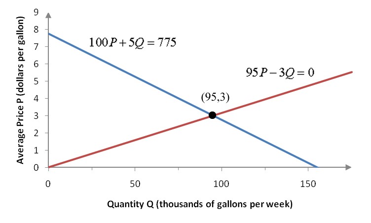
Figure 1 – A graph of the system in Section 2.1.
In Example 7 of Section 2.1, the solution (Q, P) = (95, 3) solved the system
Although the solution to the system is two numbers, there is only one ordered pair that corresponds to the solution. On a graph, this ordered pair matches the point of intersection of two lines.
In this section, we’ll examine systems which do not fit this pattern. In one type of system, there are no places on the graph where all of the lines intersect. These systems have no solutions.
For the other type of system, the lines in the system intersect at more than one ordered pair. This means that there are several solutions to the system. These systems have nonunique solutions. At the end of this section, we’ll examine how to mix different grade of ethanol to obtain a different grade of ethanol.
Read in Section 2.3
Section 2.3 Workbook (PDF) – 9/2/19
In Section 2.1, we solved several systems of linear equations by graphing each linear equation in the system. The solution to the system is any ordered pair that satisfies all of the equations. On the graph, this ordered pair is the point where all of the equations intersect.
Using a graph to find a point of intersection has limitations. If the graph is on a piece of paper, it is difficult to accurately locate the point of intersection using the scales on the axes of the graph. If you constructed the graph, you have to be extremely careful and precise to get a valid approximate answer.
A graphing calculator can draw a more accurate graph (as long as you enter the equations correctly), but the algorithms in the calculator are approximate. This means that the location of the point of intersection may be exact or it may be very close to the exact point of intersection.
Suppose we want to solve the system of linear equations
To solve this system graphically, we need to solve each linear equation for y. The first equation is already solved for y. To solve the second equation for y,
Let’s look at a graph the system to find the point of intersection.
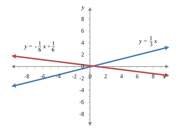
Figure 1 – A graph of a system whose point of intersection is about (0.5, 0).
From the graph, the solution to the system looks to be approximately (0.5, 0). We can check this solution by substituting x = 0.5 and y = 0 and into the original system of equations:
Since neither equation is true, the estimate of the point of intersection is not exact. To find an exact solution, we’ll need to use an algebraic strategy to solve the system of equations.
Read in Section 2.2
Section 2.2 Workbook (PDF) – 9/2/19
Watch Video Playlist
In sections 1.1 through 1.3, we considered functions of one independent variable. The cost, revenue, and profit, were each a function of some quantity Q. If we knew the quantity Q produced and sold, we could use these functions to compute the corresponding cost, revenue and profit at those production levels. As long as we deal solely with one product and the cost, revenue, and profit involved with that product, a function of one variable is adequate. But the total cost, revenue, and profit for a business may come from many products. Each of these products may have its own costs and prices. Using this information we can formulate cost, revenue and profit functions of several variables. Each of these variables represents a quantity of a different product produced and sold by the business.
In this section we’ll learn how to extend what we have learned about a function of a single independent variable to functions of several independent variables.
Read in Section 1.4